57 figures and 5 animations. Every curve is computed from a published relation or model; the source line sits under each figure. Figures that use representative values are marked as such on the figure itself.
Earthquake engineering and structural dynamics
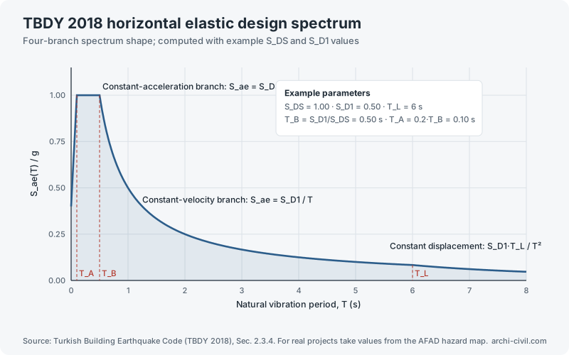
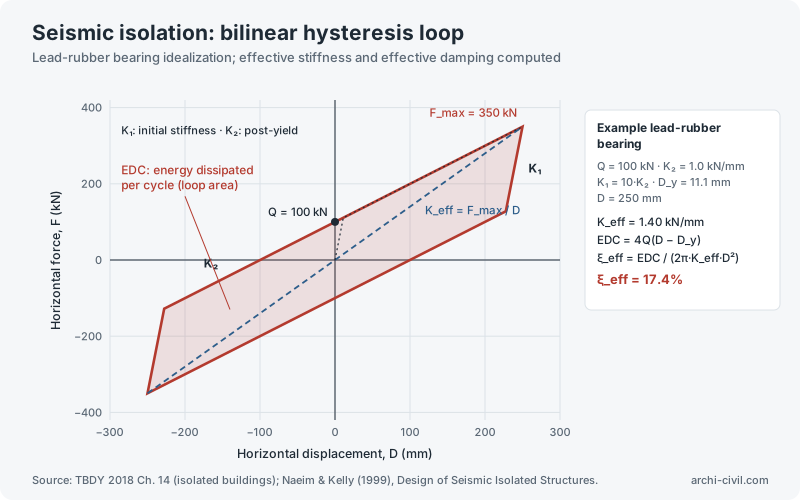
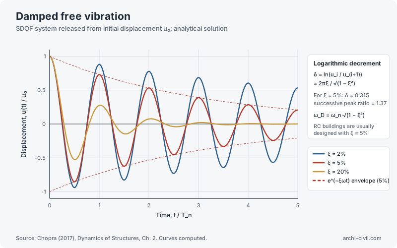
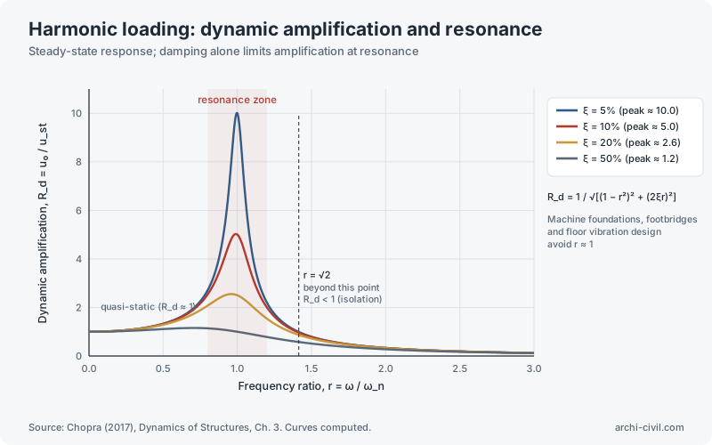
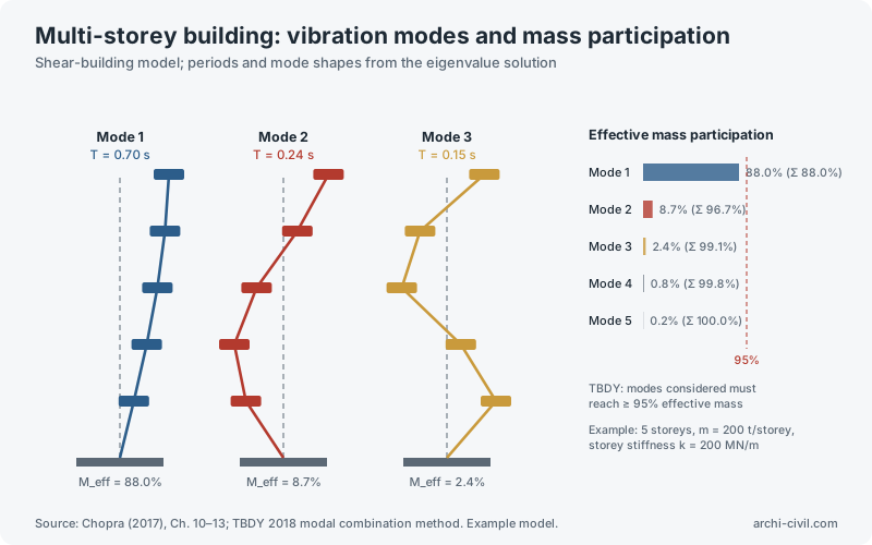
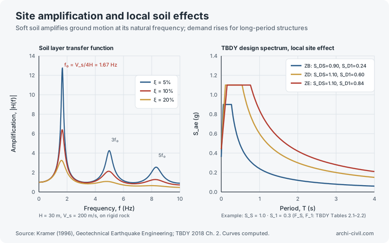
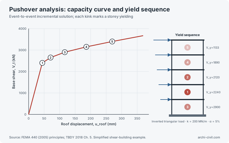
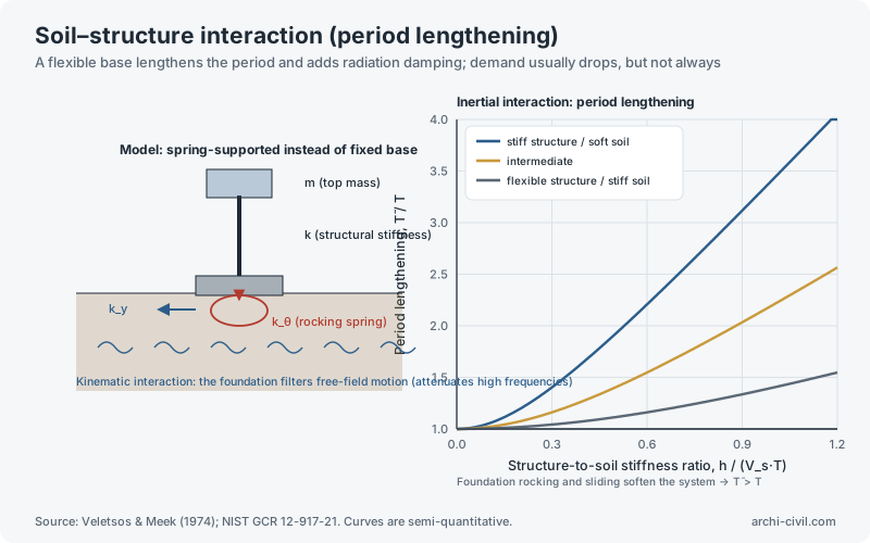
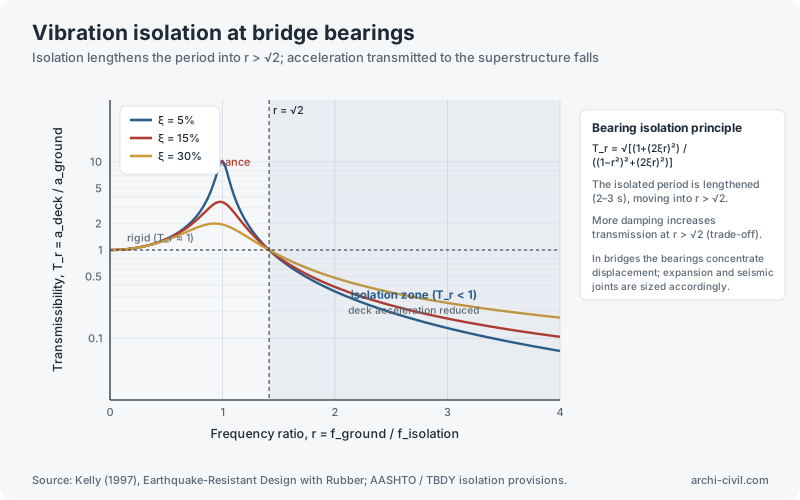
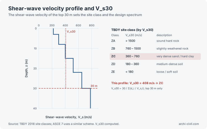
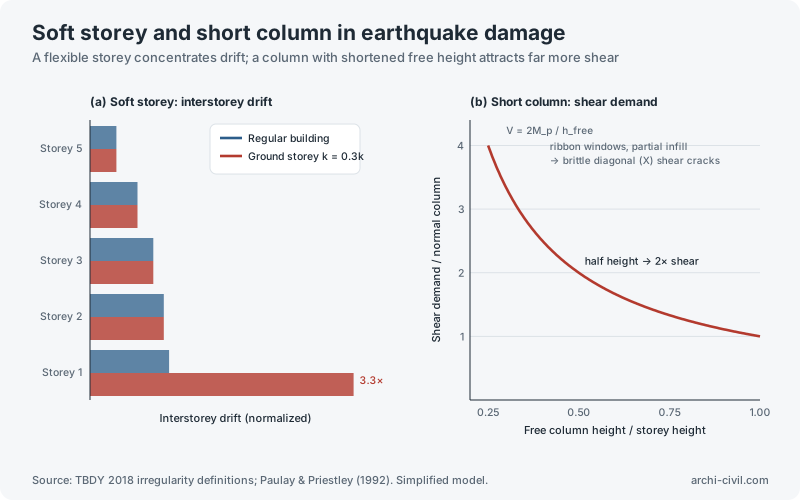
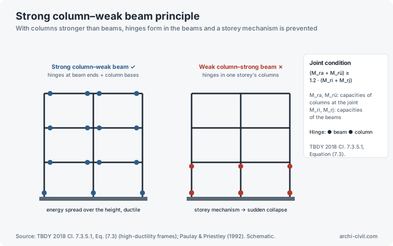
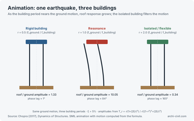
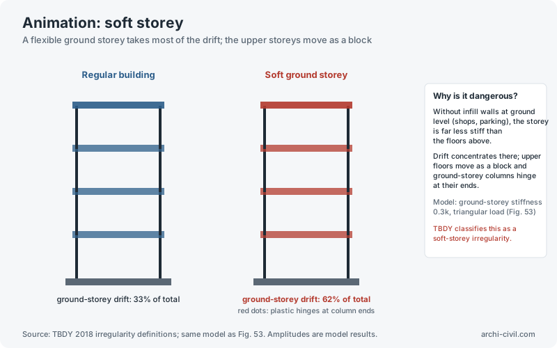
Figure 2.TBDY 2018 horizontal elastic design spectrumSource: Turkish Building Earthquake Code (TBDY 2018), Sec. 2.3.4. For real projects take values from the AFAD hazard map.Open the related tool →Figure 19.Seismic isolation: bilinear hysteresis loopSource: TBDY 2018 Ch. 14 (isolated buildings); Naeim & Kelly (1999), Design of Seismic Isolated Structures.Open the related tool →Figure 23.Damped free vibrationSource: Chopra (2017), Dynamics of Structures, Ch. 2. Curves computed.Open the related tool →Figure 24.Harmonic loading: dynamic amplification and resonanceSource: Chopra (2017), Dynamics of Structures, Ch. 3. Curves computed.Open the related tool →Figure 25.Multi-storey building: vibration modes and mass participationSource: Chopra (2017), Ch. 10–13; TBDY 2018 modal combination method. Example model.Open the related tool →Figure 33.Site amplification and local soil effectsSource: Kramer (1996), Geotechnical Earthquake Engineering; TBDY 2018 Ch. 2. Curves computed.Open the related tool →Figure 35.Pushover analysis: capacity curve and yield sequenceSource: FEMA 440 (2005) principles; TBDY 2018 Ch. 5. Simplified shear-building example.Open the related tool →Figure 38.Soil–structure interaction (period lengthening)Source: Veletsos & Meek (1974); NIST GCR 12-917-21. Curves are semi-quantitative.Open the related tool →Figure 41.Vibration isolation at bridge bearingsSource: Kelly (1997), Earthquake-Resistant Design with Rubber; AASHTO / TBDY isolation provisions.Open the related tool →Figure 43.Shear-wave velocity profile and V_s30Source: TBDY 2018 site classes; ASCE 7 uses a similar scheme. V_s30 computed.Open the related tool →Figure 53.Soft storey and short column in earthquake damageSource: TBDY 2018 irregularity definitions; Paulay & Priestley (1992). Simplified model.Open the related tool →Figure 54.Strong column–weak beam principleSource: TBDY 2018 Cl. 7.3.5.1, Eq. (7.3) (high-ductility frames); Paulay & Priestley (1992). Schematic.Open the related tool →AnimationAnimation A1.One earthquake, three buildingsSource: Chopra (2017), Dynamics of Structures. SMIL animation with motion computed from the formula.Open the related tool →AnimationAnimation A5.Soft storeySource: TBDY 2018 irregularity definitions; same model as Fig. 53. Amplitudes are model results.Open the related tool →
Reinforced concrete and steel
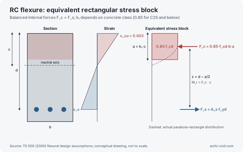
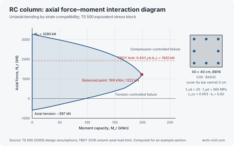
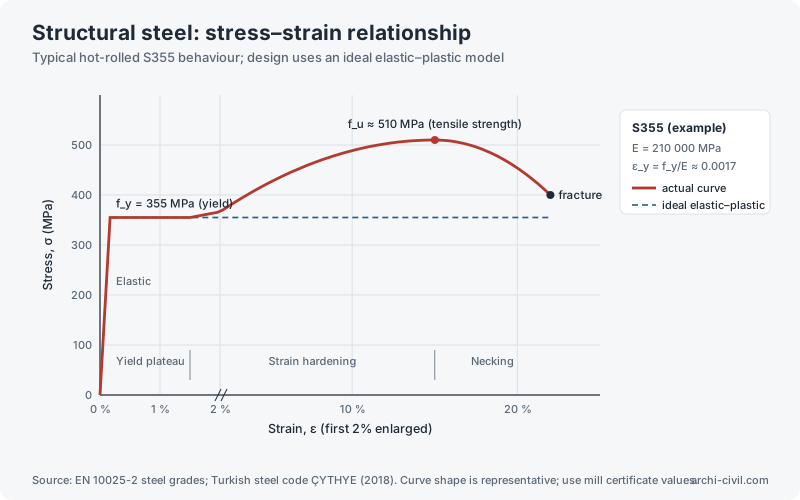
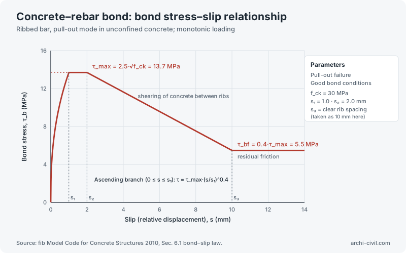
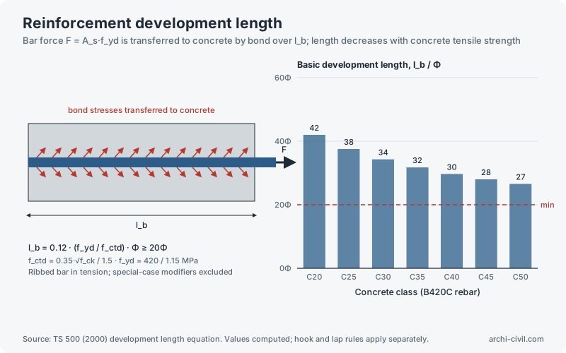
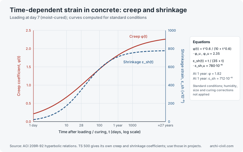
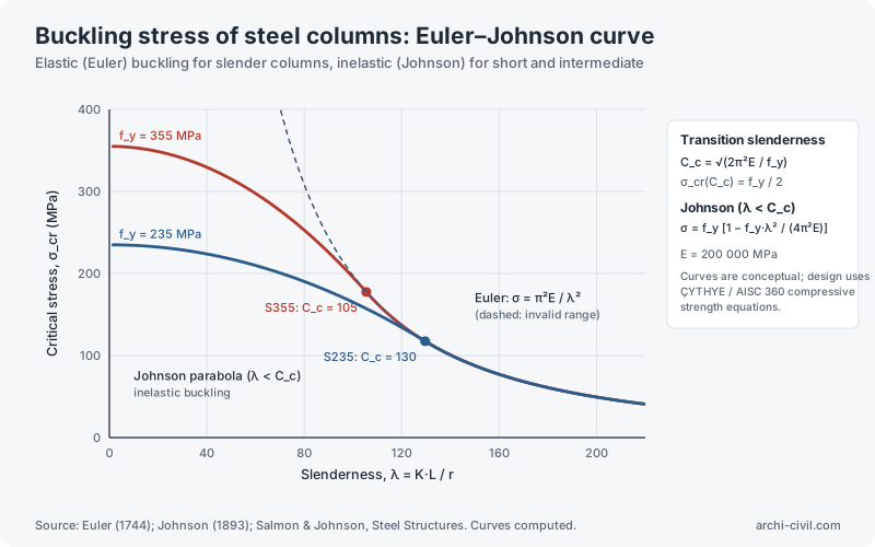
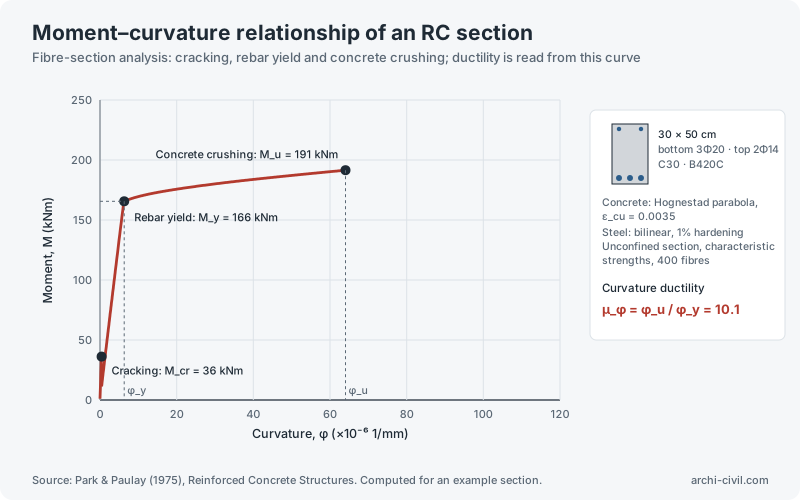
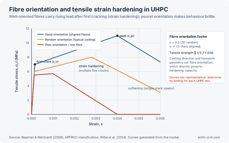
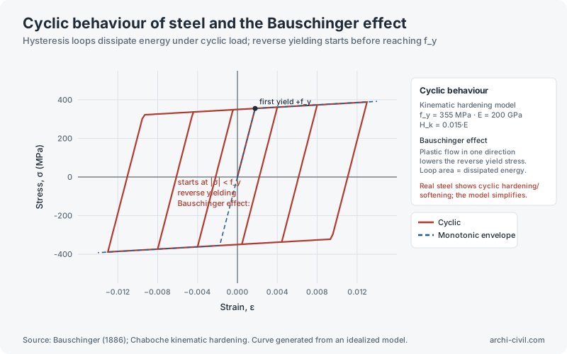
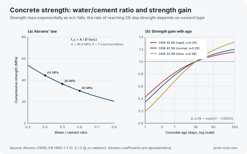
Figure 3.RC flexure: equivalent rectangular stress blockSource: TS 500 (2000) flexural design assumptions; conceptual drawing, not to scale.Open the related tool →Figure 9.RC column: axial force–moment interaction diagramSource: TS 500 (2000) design assumptions; TBDY 2018 column axial load limit. Computed for an example section.Open the related tool →Figure 10.Structural steel: stress–strain relationshipSource: EN 10025-2 steel grades; Turkish steel code ÇYTHYE (2018). Curve shape is representative; use mill certificate values.Open the related tool →Figure 17.Concrete–rebar bond: bond stress–slip relationshipSource: fib Model Code for Concrete Structures 2010, Sec. 6.1 bond–slip law.Open the related tool →Figure 18.Reinforcement development lengthSource: TS 500 (2000) development length equation. Values computed; hook and lap rules apply separately.Open the related tool →Figure 20.Time-dependent strain in concrete: creep and shrinkageSource: ACI 209R-92 hyperbolic relations. TS 500 gives its own creep and shrinkage coefficients; use those in projects.Open the related tool →Figure 29.Buckling stress of steel columns: Euler–Johnson curveSource: Euler (1744); Johnson (1893); Salmon & Johnson, Steel Structures. Curves computed.Open the related tool →Figure 34.Moment–curvature relationship of an RC sectionSource: Park & Paulay (1975), Reinforced Concrete Structures. Computed for an example section.Open the related tool →Figure 39.Fibre orientation and tensile strain hardening in UHPCSource: Naaman & Reinhardt (2006), HPFRCC classification; Wille et al. (2014). Curves generated from the model.Open the related tool →Figure 42.Cyclic behaviour of steel and the Bauschinger effectSource: Bauschinger (1886); Chaboche kinematic hardening. Curve generated from an idealized model.Open the related tool →Figure 55.Concrete strength: water/cement ratio and strength gainSource: Abrams (1918); EN 1992-1-1 Cl. 3.1.2 (β_cc relation). Abrams coefficients are representative.Open the related tool →
Statics and mechanics of materials
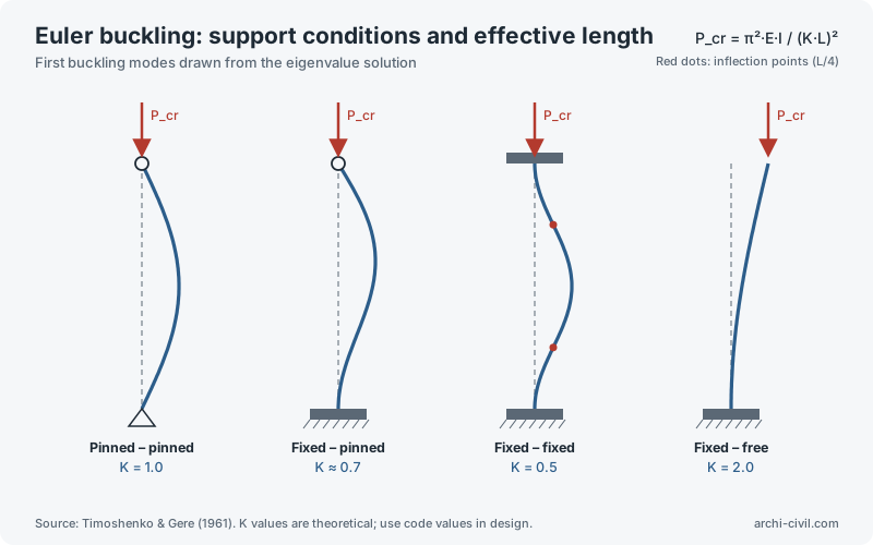
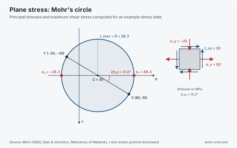
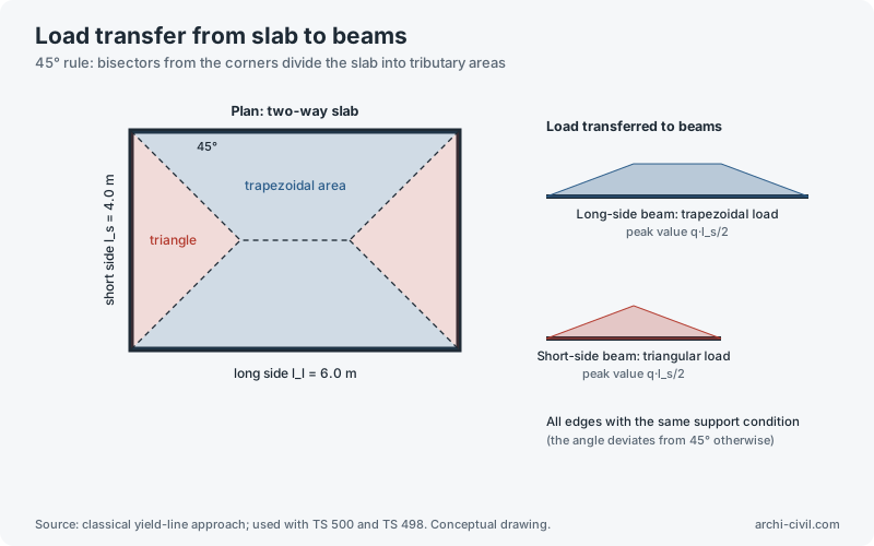
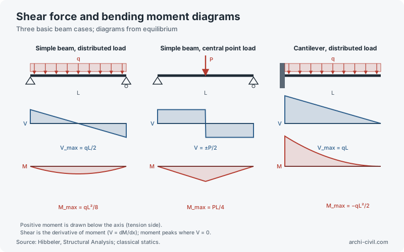
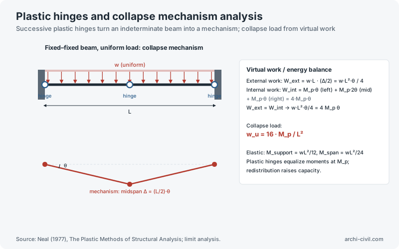
Figure 4.Euler buckling: support conditions and effective lengthSource: Timoshenko & Gere (1961). K values are theoretical; use code values in design.Open the related tool →Figure 11.Plane stress: Mohr's circleSource: Mohr (1882); Beer & Johnston, Mechanics of Materials. τ axis drawn positive downward.Open the related tool →Figure 12.Load transfer from slab to beamsSource: classical yield-line approach; used with TS 500 and TS 498. Conceptual drawing.Open the related tool →Figure 28.Shear force and bending moment diagramsSource: Hibbeler, Structural Analysis; classical statics.Open the related tool →Figure 45.Plastic hinges and collapse mechanism analysisSource: Neal (1977), The Plastic Methods of Structural Analysis; limit analysis.Open the related tool →
Geotechnics and foundations
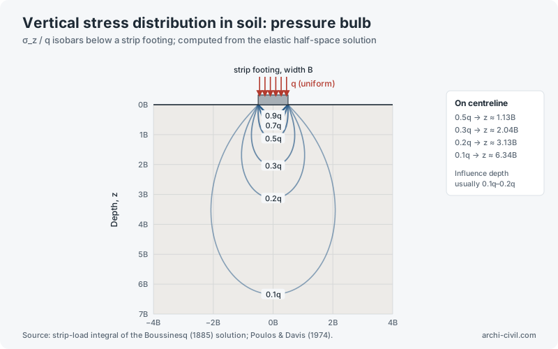
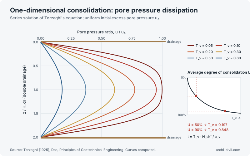
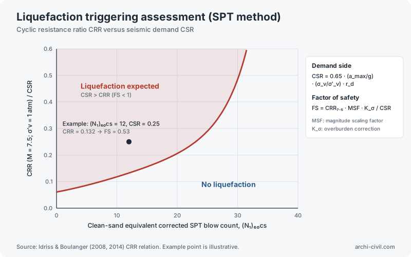
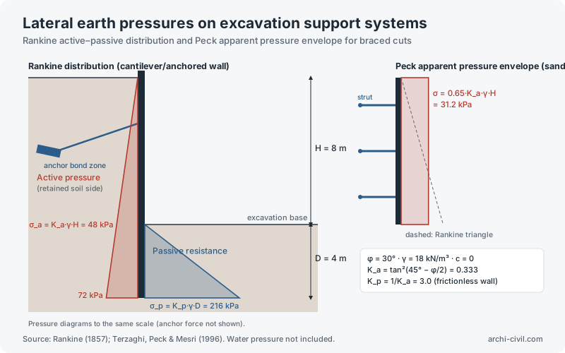
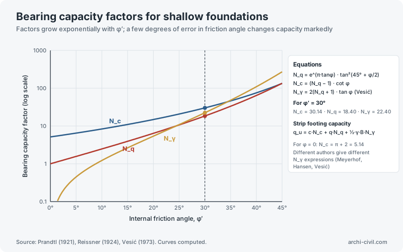
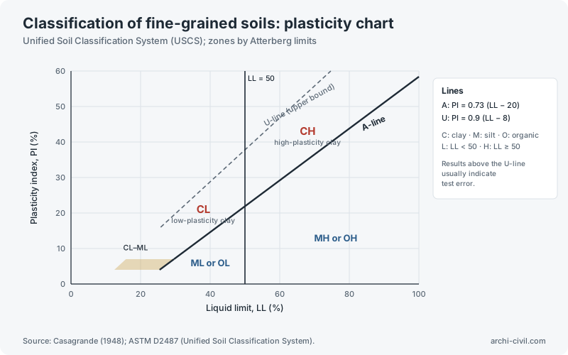
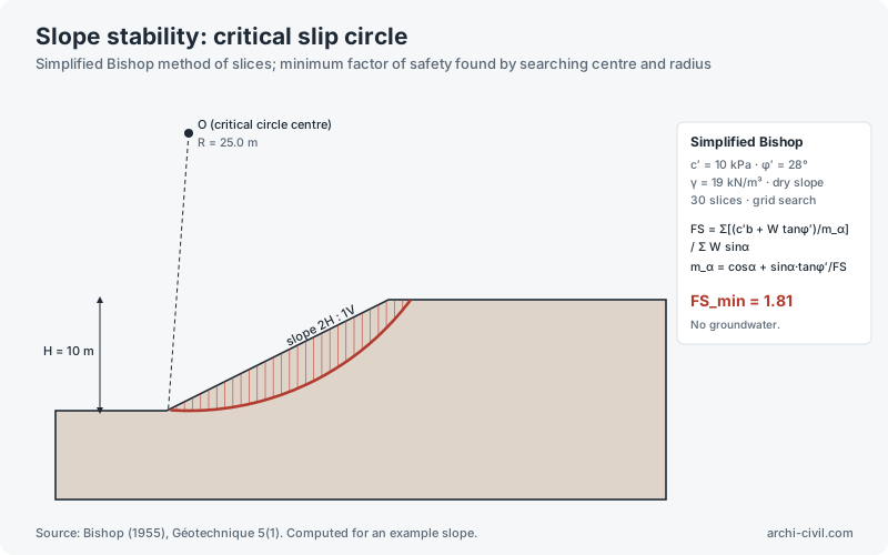
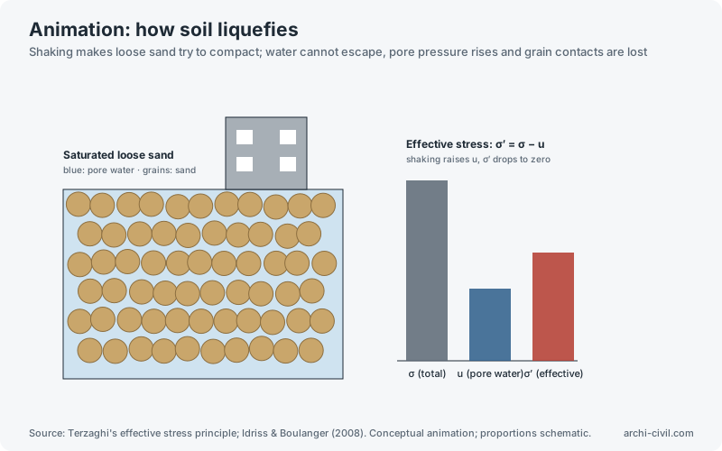
Figure 13.Vertical stress distribution in soil: pressure bulbSource: strip-load integral of the Boussinesq (1885) solution; Poulos & Davis (1974).Open the related tool →Figure 14.One-dimensional consolidation: pore pressure dissipationSource: Terzaghi (1925); Das, Principles of Geotechnical Engineering. Curves computed.Open the related tool →Figure 15.Liquefaction triggering assessment (SPT method)Source: Idriss & Boulanger (2008, 2014) CRR relation. Example point is illustrative.Open the related tool →Figure 22.Lateral earth pressures on excavation support systemsSource: Rankine (1857); Terzaghi, Peck & Mesri (1996). Water pressure not included.Open the related tool →Figure 26.Bearing capacity factors for shallow foundationsSource: Prandtl (1921), Reissner (1924), Vesić (1973). Curves computed.Open the related tool →Figure 30.Classification of fine-grained soils: plasticity chartSource: Casagrande (1948); ASTM D2487 (Unified Soil Classification System).Open the related tool →Figure 31.Slope stability: critical slip circleSource: Bishop (1955), Géotechnique 5(1). Computed for an example slope.Open the related tool →AnimationAnimation A4.How soil liquefiesSource: Terzaghi's effective stress principle; Idriss & Boulanger (2008). Conceptual animation; proportions schematic.Open the related tool →
Protective structures
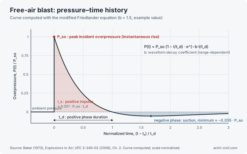
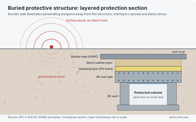
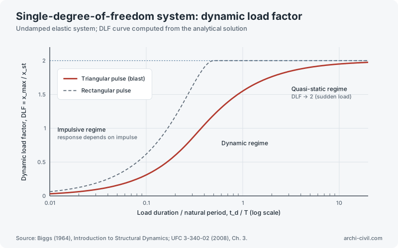
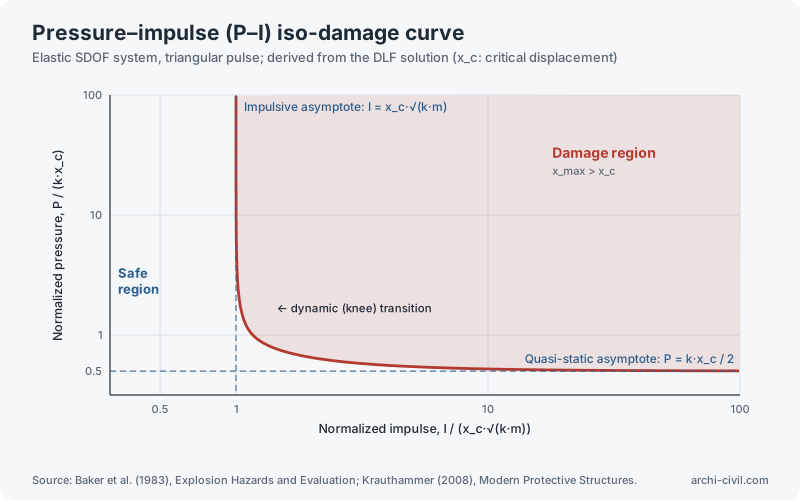
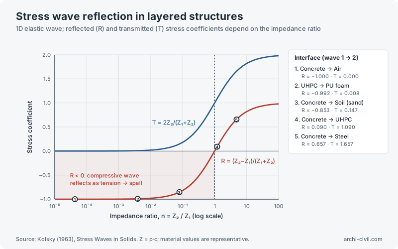
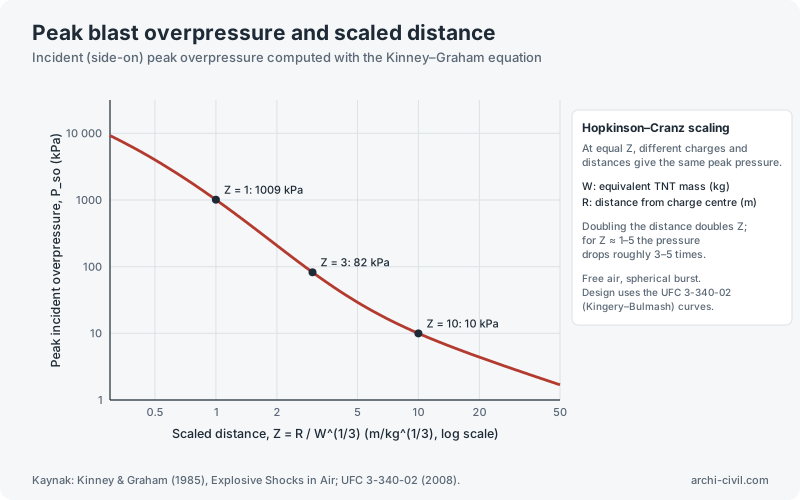
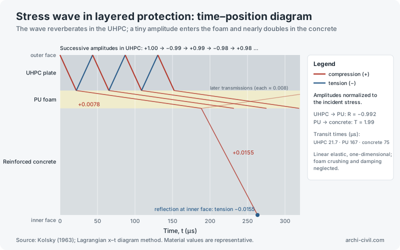
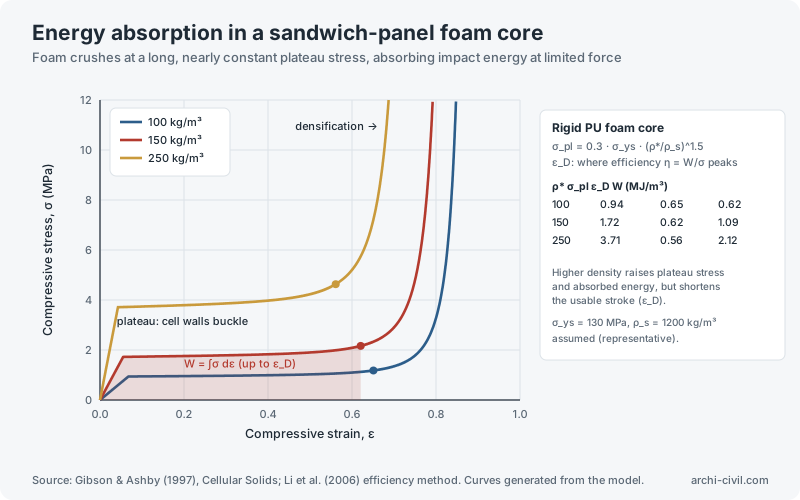
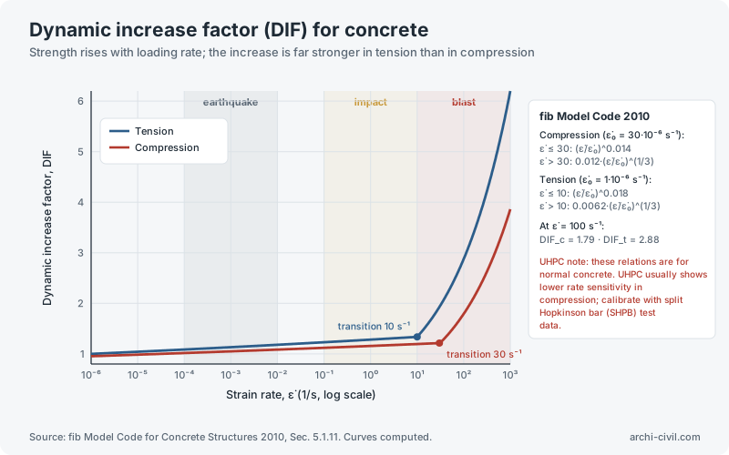
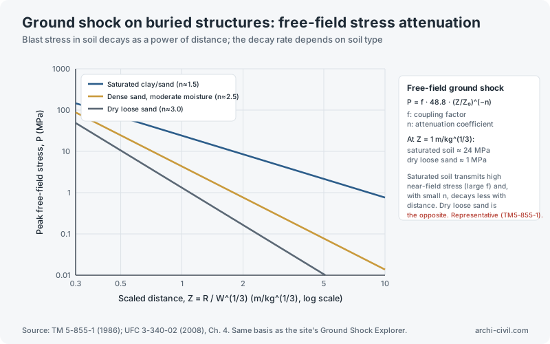
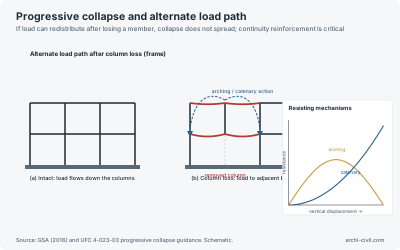
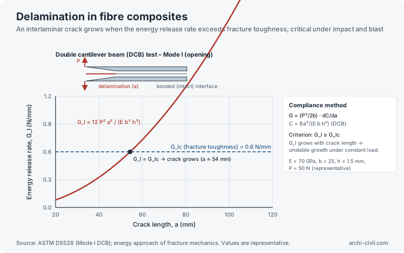
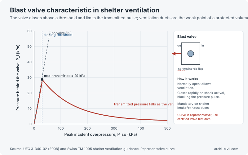
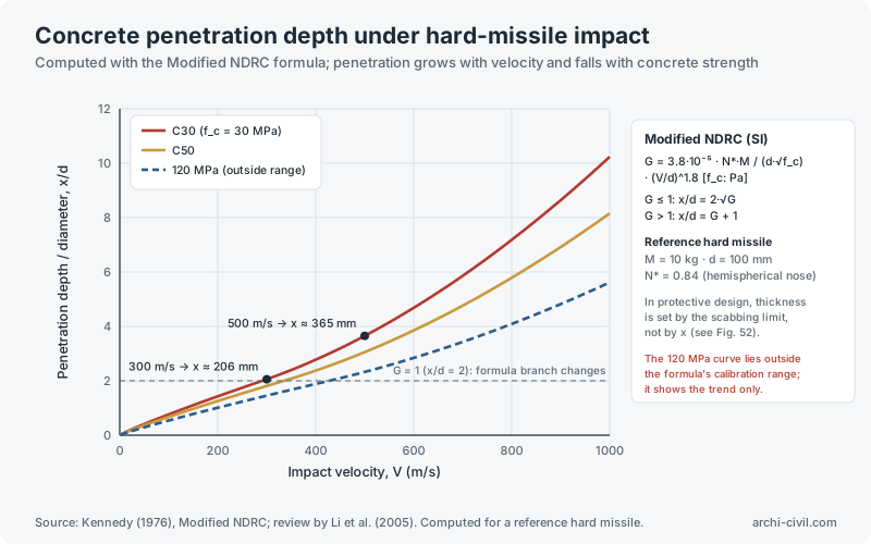
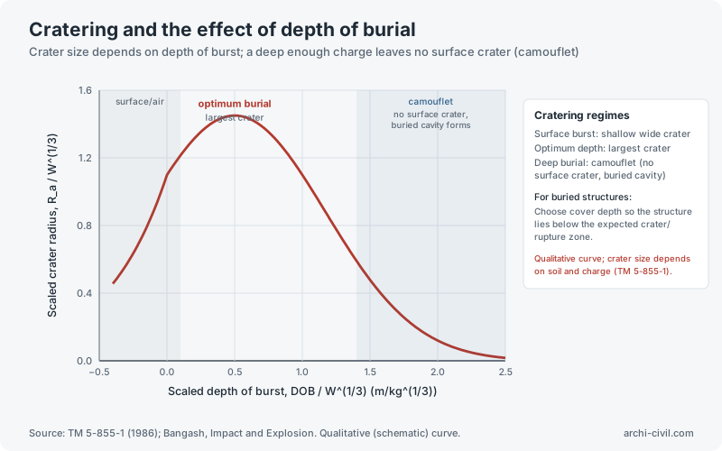
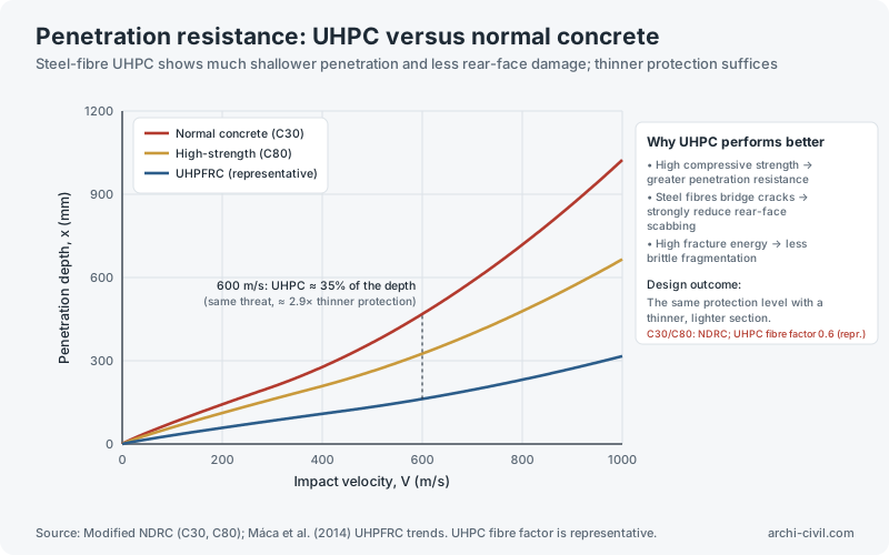
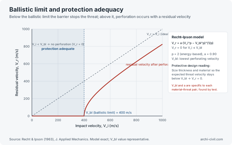
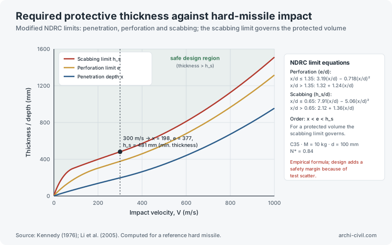
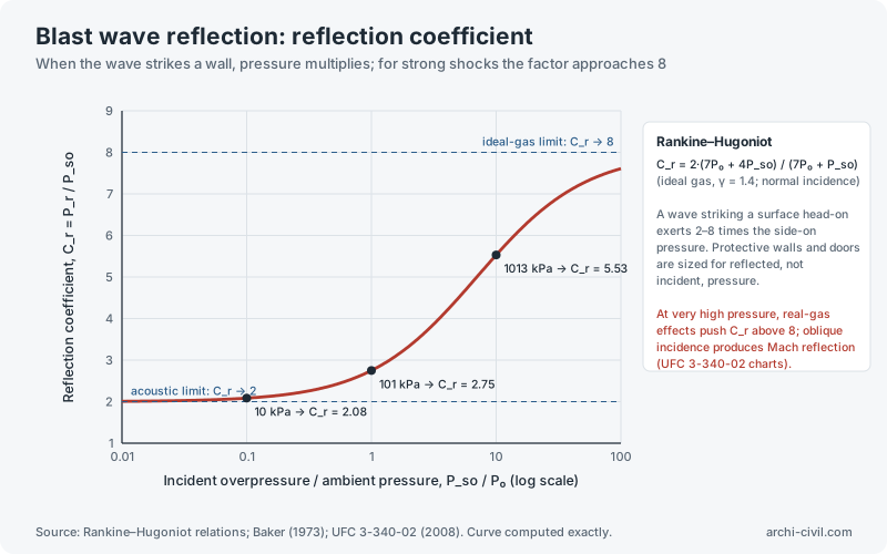
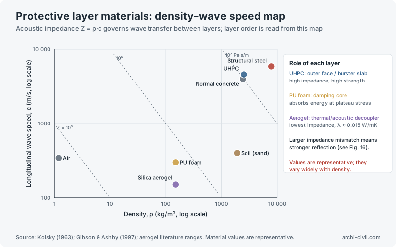
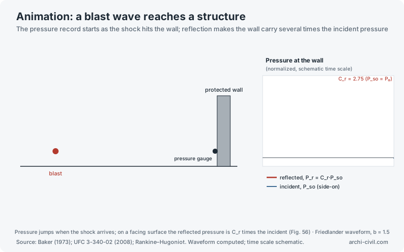
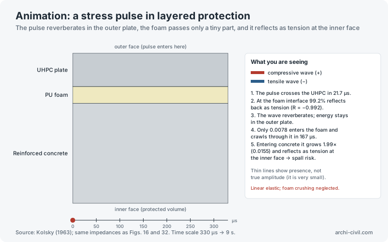
Figure 1.Free-air blast: pressure–time historySource: Baker (1973), Explosions in Air; UFC 3-340-02 (2008), Ch. 2. Curve computed; scale normalized.Open the related tool →Figure 6.Buried protective structure: layered protection sectionSource: UFC 3-340-02 (2008) principles. Conceptual section; layer thicknesses not to scale.Open the related tool →Figure 7.Single-degree-of-freedom system: dynamic load factorSource: Biggs (1964), Introduction to Structural Dynamics; UFC 3-340-02 (2008), Ch. 3.Open the related tool →Figure 8.Pressure–impulse (P–I) iso-damage curveSource: Baker et al. (1983), Explosion Hazards and Evaluation; Krauthammer (2008), Modern Protective Structures.Open the related tool →Figure 16.Stress wave reflection in layered structuresSource: Kolsky (1963), Stress Waves in Solids. Z = ρ·c; material values are representative.Open the related tool →Figure 27.Peak blast overpressure and scaled distanceKaynak: Kinney & Graham (1985), Explosive Shocks in Air; UFC 3-340-02 (2008).Open the related tool →Figure 32.Stress wave in layered protection: time–position diagramSource: Kolsky (1963); Lagrangian x–t diagram method. Material values are representative.Open the related tool →Figure 36.Energy absorption in a sandwich-panel foam coreSource: Gibson & Ashby (1997), Cellular Solids; Li et al. (2006) efficiency method. Curves generated from the model.Open the related tool →Figure 37.Dynamic increase factor (DIF) for concreteSource: fib Model Code for Concrete Structures 2010, Sec. 5.1.11. Curves computed.Open the related tool →Figure 40.Ground shock on buried structures: free-field stress attenuationSource: TM 5-855-1 (1986); UFC 3-340-02 (2008), Ch. 4. Same basis as the site's Ground Shock Explorer.Open the related tool →Figure 44.Progressive collapse and alternate load pathSource: GSA (2016) and UFC 4-023-03 progressive collapse guidance. Schematic.Open the related tool →Figure 46.Delamination in fibre compositesSource: ASTM D5528 (Mode I DCB); energy approach of fracture mechanics. Values are representative.Open the related tool →Figure 47.Blast valve characteristic in shelter ventilationSource: UFC 3-340-02 (2008) and Swiss TM 1995 shelter ventilation guidance. Representative curve.Open the related tool →Figure 48.Concrete penetration depth under hard-missile impactSource: Kennedy (1976), Modified NDRC; review by Li et al. (2005). Computed for a reference hard missile.Open the related tool →Figure 49.Cratering and the effect of depth of burialSource: TM 5-855-1 (1986); Bangash, Impact and Explosion. Qualitative (schematic) curve.Open the related tool →Figure 50.Penetration resistance: UHPC versus normal concreteSource: Modified NDRC (C30, C80); Máca et al. (2014) UHPFRC trends. UHPC fibre factor is representative.Open the related tool →Figure 51.Ballistic limit and protection adequacySource: Recht & Ipson (1963), J. Applied Mechanics. Model exact; V_bl value representative.Open the related tool →Figure 52.Required protective thickness against hard-missile impactSource: Kennedy (1976); Li et al. (2005). Computed for a reference hard missile.Open the related tool →Figure 56.Blast wave reflection: reflection coefficientSource: Rankine–Hugoniot relations; Baker (1973); UFC 3-340-02 (2008). Curve computed exactly.Open the related tool →Figure 57.Protective layer materials: density–wave speed mapSource: Kolsky (1963); Gibson & Ashby (1997); aerogel literature ranges. Material values are representative.Open the related tool →AnimationAnimation A2.A blast wave reaches a structureSource: Baker (1973); UFC 3-340-02 (2008); Rankine–Hugoniot. Waveform computed; time scale schematic.Open the related tool →AnimationAnimation A3.A stress pulse in layered protectionSource: Kolsky (1963); same impedances as Figs. 16 and 32. Time scale 330 µs → 9 s.Open the related tool →
Building physics
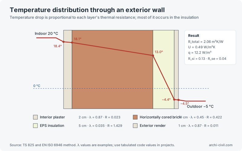
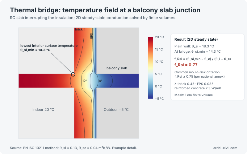
Figure 5.Temperature distribution through an exterior wallSource: TS 825 and EN ISO 6946 method. λ values are examples; use tabulated code values in projects.Open the related tool →Figure 21.Thermal bridge: temperature field at a balcony slab junctionSource: EN ISO 10211 method; R_si = 0.13, R_se = 0.04 m²K/W. Example detail.Open the related tool →