75 figures and 9 animations. Every curve is computed from a published relation or model; the source line sits under each figure. Figures that use representative values are marked as such on the figure itself.
Interactive charts — change the values yourself
These charts are computed live in your browser. Where the site has a calculation engine (spectrum, bearing capacity, blast) the chart calls it directly; the others are verified closed-form relations.
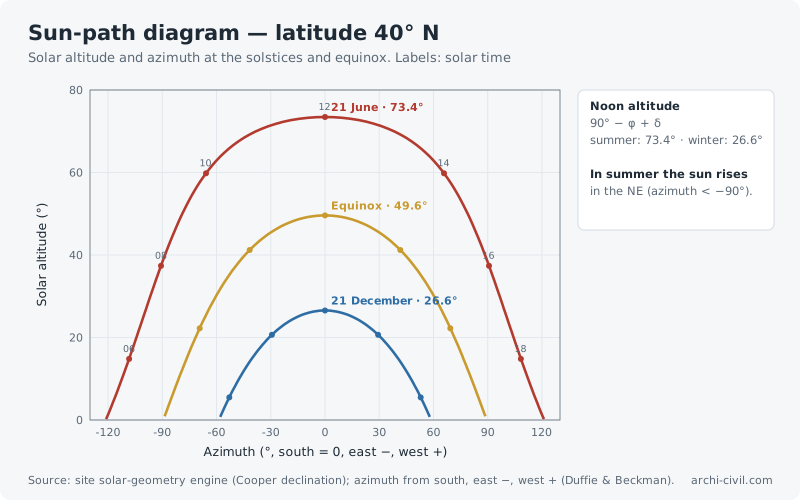
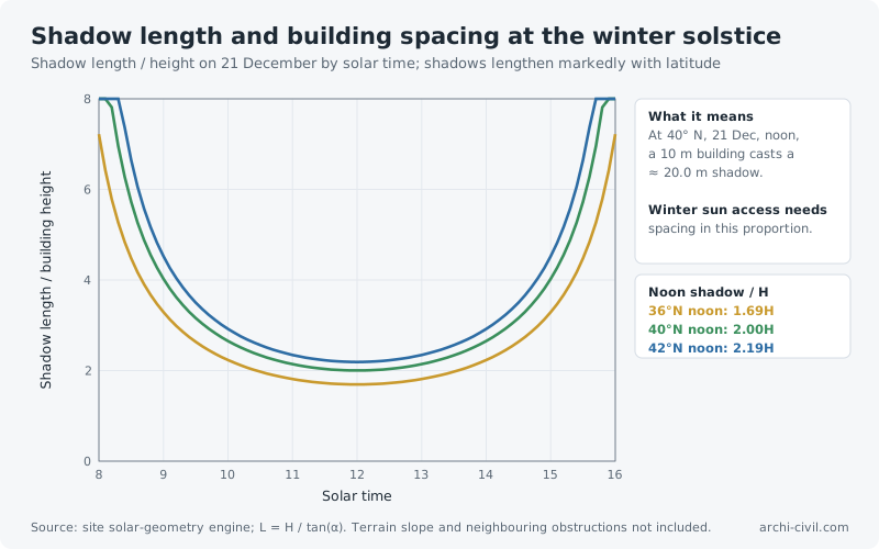
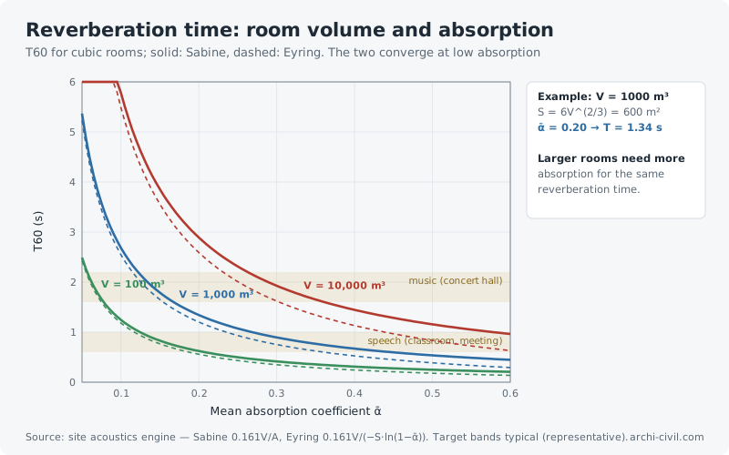
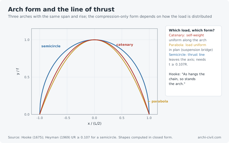
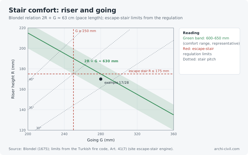
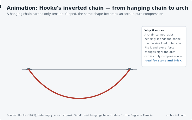
Figure 64.Sun-path diagram — latitude 40° NSolar altitude and azimuth at the solstices and equinox. Labels: solar timeSource: site solar-geometry engine (Cooper declination); azimuth from south, east −, west + (Duffie & Beckman).Open the related page →Figure 65.Shadow length and building spacing at the winter solsticeShadow length / height on 21 December by solar time; shadows lengthen markedly with latitudeSource: site solar-geometry engine; L = H / tan(α). Terrain slope and neighbouring obstructions not included.Open the related page →Figure 66.Reverberation time: room volume and absorptionT60 for cubic rooms; solid: Sabine, dashed: Eyring. The two converge at low absorptionSource: site acoustics engine — Sabine 0.161V/A, Eyring 0.161V/(−S·ln(1−ᾱ)). Target bands typical (representative).Open the related page →Figure 67.Arch form and the line of thrustThree arches with the same span and rise; the compression-only form depends on how the load is distributedSource: Hooke (1675); Heyman (1969) t/R ≥ 0.107 for a semicircle. Shapes computed in closed form.Open the related page →Figure 68.Stair comfort: riser and goingBlondel relation 2R + G ≈ 63 cm (pace length); escape-stair limits from the regulationSource: Blondel (1675); limits from the Turkish fire code, Art. 41(7) (site escape-stair engine).Open the related page →AnimationAnimation A9.Hooke's inverted chain — from hanging chain to archA hanging chain carries only tension; flipped, the same shape becomes an arch in pure compressionSource: Hooke (1675); catenary y = a·cosh(x/a). Gaudí used hanging-chain models for the Sagrada Família.Open the related page →
Earthquake engineering and structural dynamics
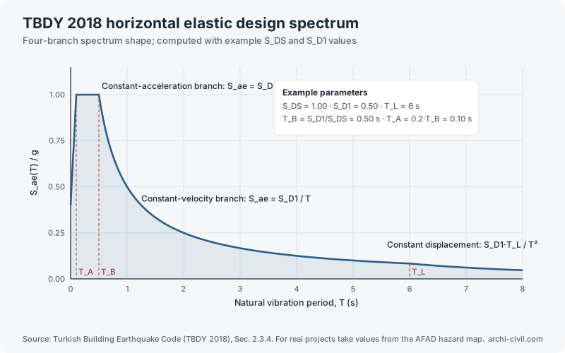
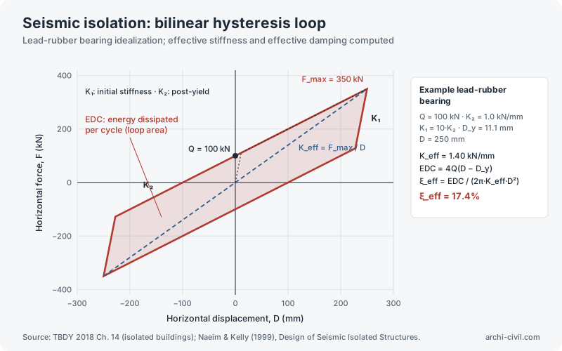
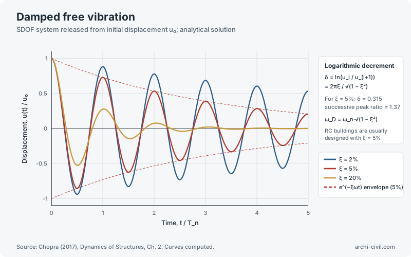
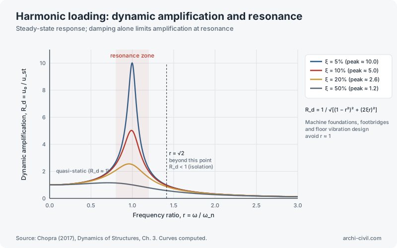
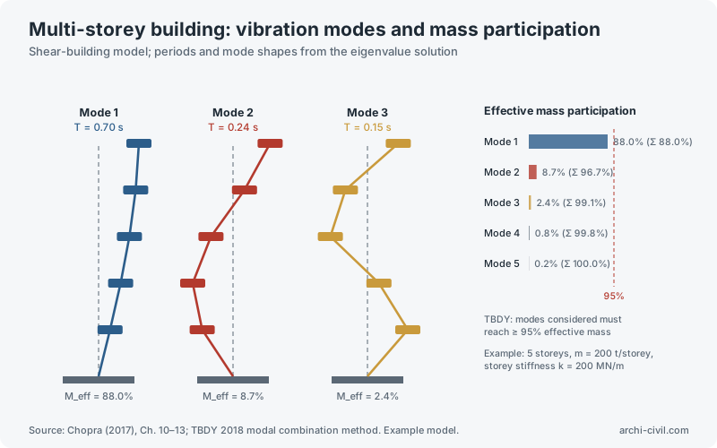
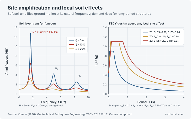
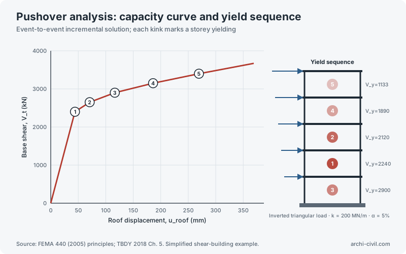
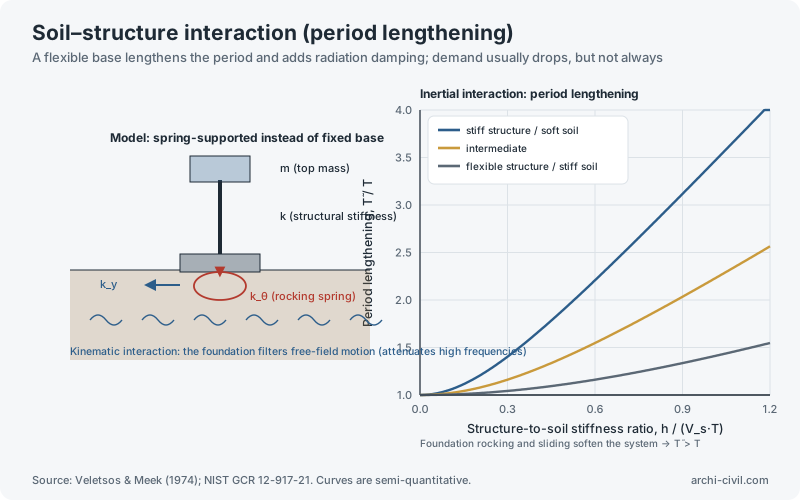
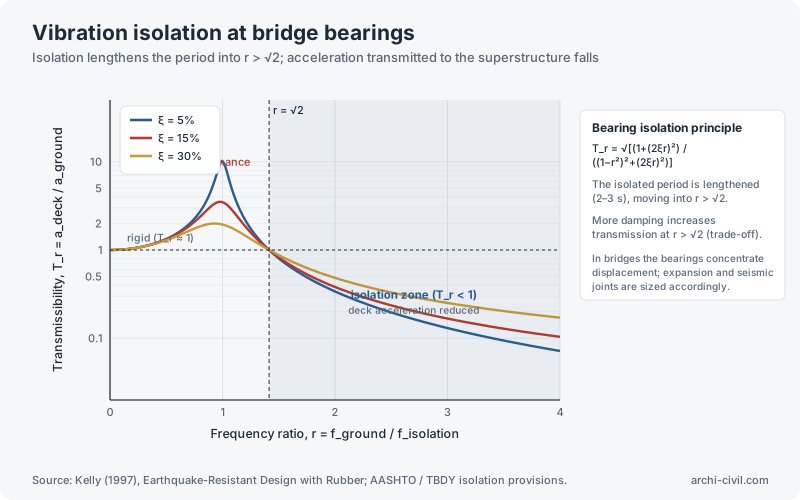
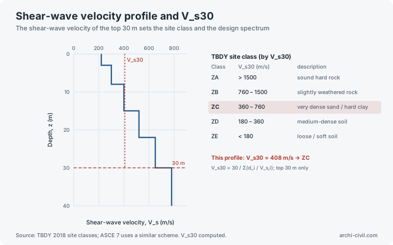
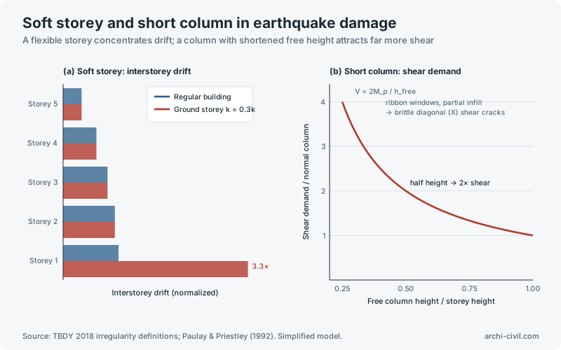
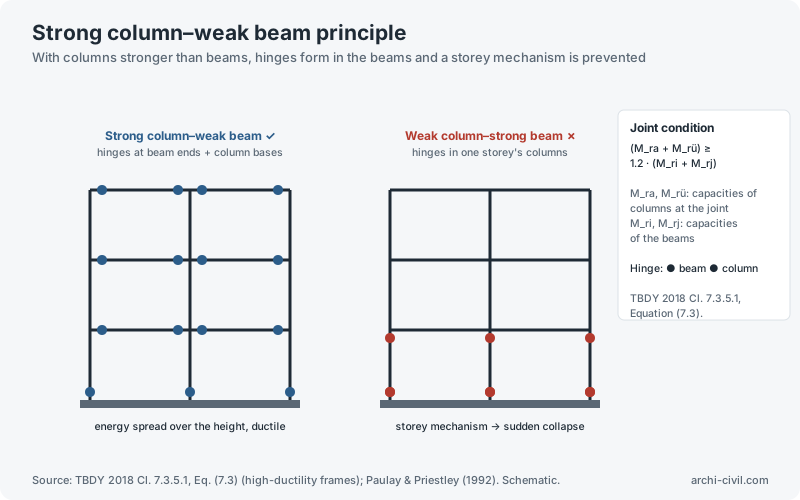
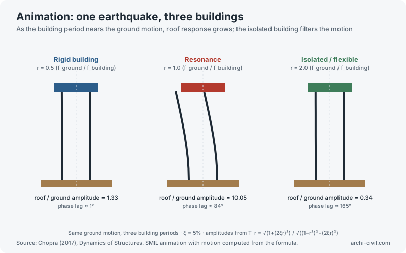
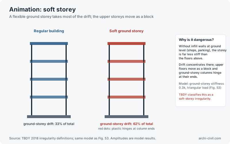
Figure 2.TBDY 2018 horizontal elastic design spectrumFour-branch spectrum shape; computed with example S_DS and S_D1 valuesSource: Turkish Building Earthquake Code (TBDY 2018), Sec. 2.3.4. For real projects take values from the AFAD hazard map.Open the related tool →Figure 19.Seismic isolation: bilinear hysteresis loopLead-rubber bearing idealization; effective stiffness and effective damping computedSource: TBDY 2018 Ch. 14 (isolated buildings); Naeim & Kelly (1999), Design of Seismic Isolated Structures.Open the related tool →Figure 23.Damped free vibrationSDOF system released from initial displacement u₀; analytical solutionSource: Chopra (2017), Dynamics of Structures, Ch. 2. Curves computed.Open the related tool →Figure 24.Harmonic loading: dynamic amplification and resonanceSteady-state response; damping alone limits amplification at resonanceSource: Chopra (2017), Dynamics of Structures, Ch. 3. Curves computed.Open the related tool →Figure 25.Multi-storey building: vibration modes and mass participationShear-building model; periods and mode shapes from the eigenvalue solutionSource: Chopra (2017), Ch. 10–13; TBDY 2018 modal combination method. Example model.Open the related tool →Figure 33.Site amplification and local soil effectsSoft soil amplifies ground motion at its natural frequency; demand rises for long-period structuresSource: Kramer (1996), Geotechnical Earthquake Engineering; TBDY 2018 Ch. 2. Curves computed.Open the related tool →Figure 35.Pushover analysis: capacity curve and yield sequenceEvent-to-event incremental solution; each kink marks a storey yieldingSource: FEMA 440 (2005) principles; TBDY 2018 Ch. 5. Simplified shear-building example.Open the related tool →Figure 38.Soil–structure interaction (period lengthening)A flexible base lengthens the period and adds radiation damping; demand usually drops, but not alwaysSource: Veletsos & Meek (1974); NIST GCR 12-917-21. Curves are semi-quantitative.Open the related tool →Figure 41.Vibration isolation at bridge bearingsIsolation lengthens the period into r > √2; acceleration transmitted to the superstructure fallsSource: Kelly (1997), Earthquake-Resistant Design with Rubber; AASHTO / TBDY isolation provisions.Open the related tool →Figure 43.Shear-wave velocity profile and V_s30The shear-wave velocity of the top 30 m sets the site class and the design spectrumSource: TBDY 2018 site classes; ASCE 7 uses a similar scheme. V_s30 computed.Open the related tool →Figure 53.Soft storey and short column in earthquake damageA flexible storey concentrates drift; a column with shortened free height attracts far more shearSource: TBDY 2018 irregularity definitions; Paulay & Priestley (1992). Simplified model.Open the related tool →Figure 54.Strong column–weak beam principleWith columns stronger than beams, hinges form in the beams and a storey mechanism is preventedSource: TBDY 2018 Cl. 7.3.5.1, Eq. (7.3) (high-ductility frames); Paulay & Priestley (1992). Schematic.Open the related tool →AnimationAnimation A1.One earthquake, three buildingsAs the building period nears the ground motion, roof response grows; the isolated building filters the motionSource: Chopra (2017), Dynamics of Structures. SMIL animation with motion computed from the formula.Open the related tool →AnimationAnimation A5.Soft storeyA flexible ground storey takes most of the drift; the upper storeys move as a blockSource: TBDY 2018 irregularity definitions; same model as Fig. 53. Amplitudes are model results.Open the related tool →
Reinforced concrete and steel
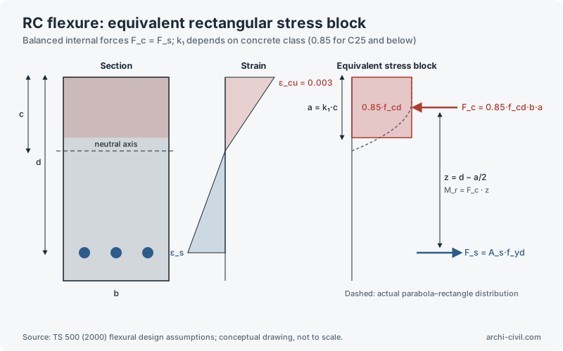
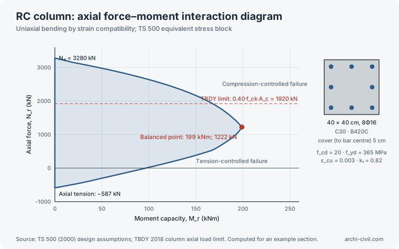
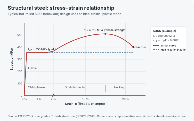
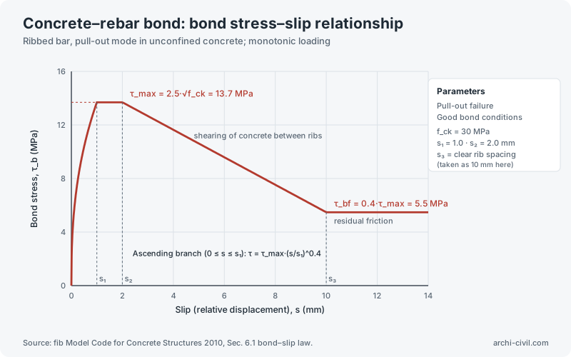
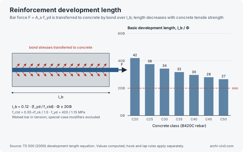
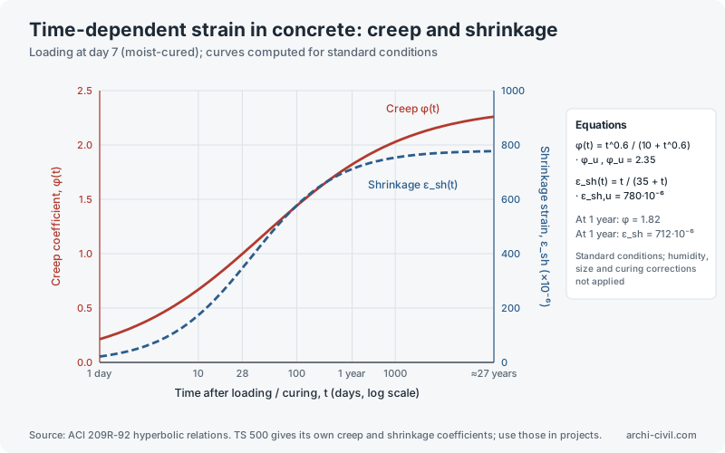
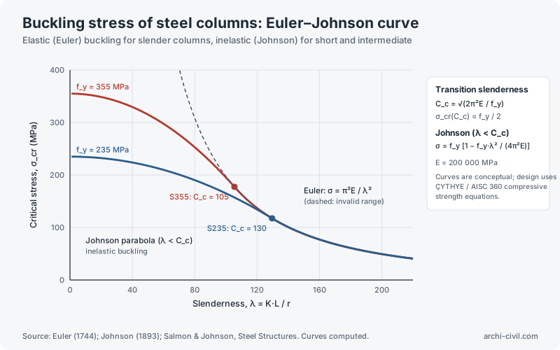
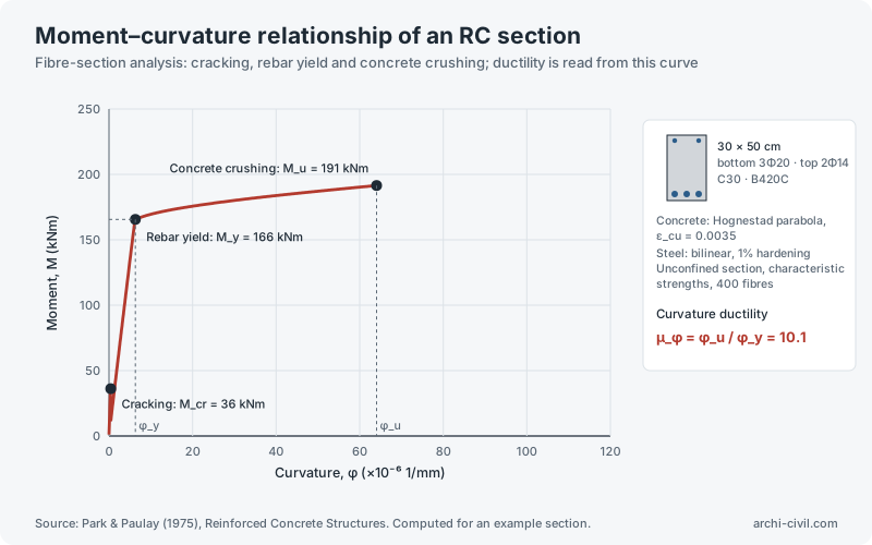
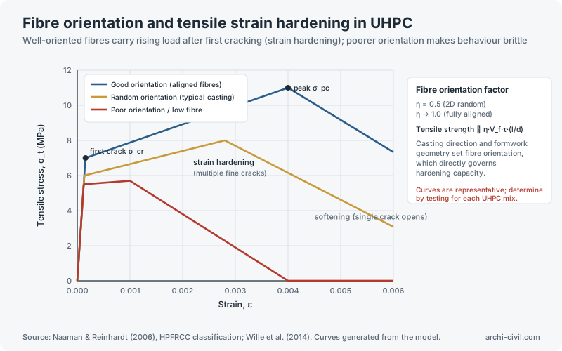
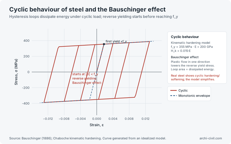
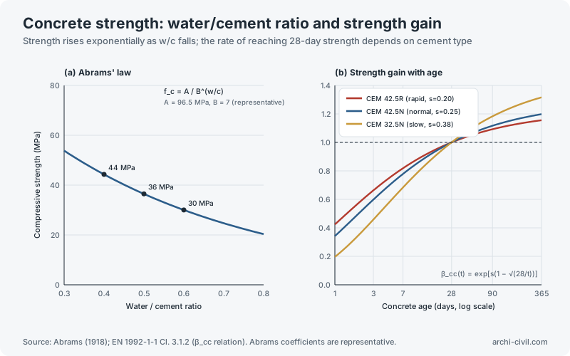
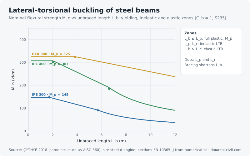
Figure 3.RC flexure: equivalent rectangular stress blockBalanced internal forces F_c = F_s; k₁ depends on concrete class (0.85 for C25 and below)Source: TS 500 (2000) flexural design assumptions; conceptual drawing, not to scale.Open the related tool →Figure 9.RC column: axial force–moment interaction diagramUniaxial bending by strain compatibility; TS 500 equivalent stress blockSource: TS 500 (2000) design assumptions; TBDY 2018 column axial load limit. Computed for an example section.Open the related tool →Figure 10.Structural steel: stress–strain relationshipTypical hot-rolled S355 behaviour; design uses an ideal elastic–plastic modelSource: EN 10025-2 steel grades; Turkish steel code ÇYTHYE (2018). Curve shape is representative; use mill certificate values.Open the related tool →Figure 17.Concrete–rebar bond: bond stress–slip relationshipRibbed bar, pull-out mode in unconfined concrete; monotonic loadingSource: fib Model Code for Concrete Structures 2010, Sec. 6.1 bond–slip law.Open the related tool →Figure 18.Reinforcement development lengthBar force F = A_s·f_yd is transferred to concrete by bond over l_b; length decreases with concrete tensile strengthSource: TS 500 (2000) development length equation. Values computed; hook and lap rules apply separately.Open the related tool →Figure 20.Time-dependent strain in concrete: creep and shrinkageLoading at day 7 (moist-cured); curves computed for standard conditionsSource: ACI 209R-92 hyperbolic relations. TS 500 gives its own creep and shrinkage coefficients; use those in projects.Open the related tool →Figure 29.Buckling stress of steel columns: Euler–Johnson curveElastic (Euler) buckling for slender columns, inelastic (Johnson) for short and intermediateSource: Euler (1744); Johnson (1893); Salmon & Johnson, Steel Structures. Curves computed.Open the related tool →Figure 34.Moment–curvature relationship of an RC sectionFibre-section analysis: cracking, rebar yield and concrete crushing; ductility is read from this curveSource: Park & Paulay (1975), Reinforced Concrete Structures. Computed for an example section.Open the related tool →Figure 39.Fibre orientation and tensile strain hardening in UHPCWell-oriented fibres carry rising load after first cracking (strain hardening); poorer orientation makes behaviour brittleSource: Naaman & Reinhardt (2006), HPFRCC classification; Wille et al. (2014). Curves generated from the model.Open the related tool →Figure 42.Cyclic behaviour of steel and the Bauschinger effectHysteresis loops dissipate energy under cyclic load; reverse yielding starts before reaching f_ySource: Bauschinger (1886); Chaboche kinematic hardening. Curve generated from an idealized model.Open the related tool →Figure 55.Concrete strength: water/cement ratio and strength gainStrength rises exponentially as w/c falls; the rate of reaching 28-day strength depends on cement typeSource: Abrams (1918); EN 1992-1-1 Cl. 3.1.2 (β_cc relation). Abrams coefficients are representative.Open the related tool →Figure 63.Lateral–torsional buckling of steel beamsNominal flexural strength M_n vs unbraced length L_b: yielding, inelastic and elastic zones (C_b = 1, S235)Source: ÇYTHYE 2018 (same structure as AISC 360), site steel-d engine; sections EN 10365, J from numerical solution.Open the related tool →
Statics and mechanics of materials
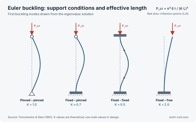
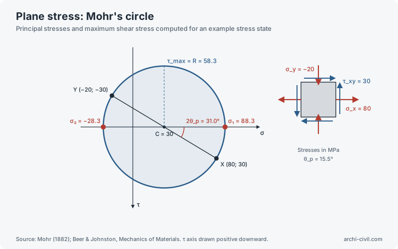
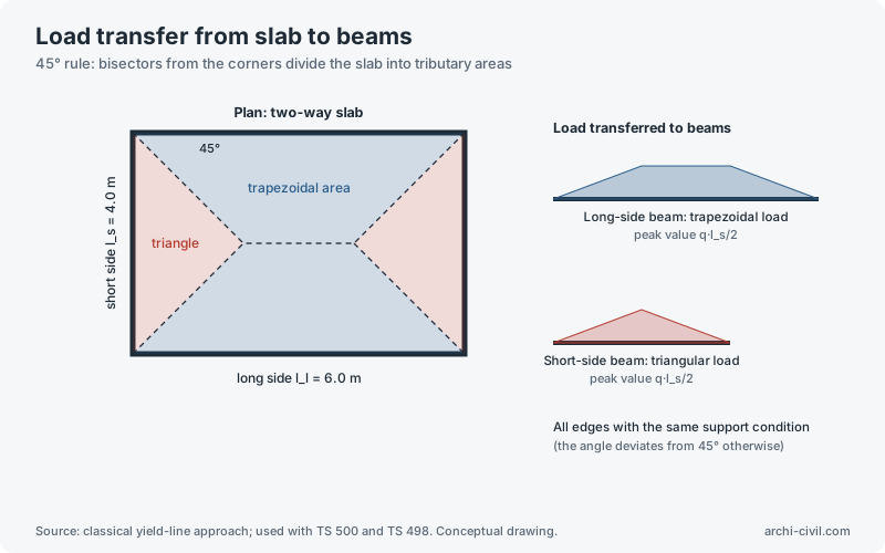
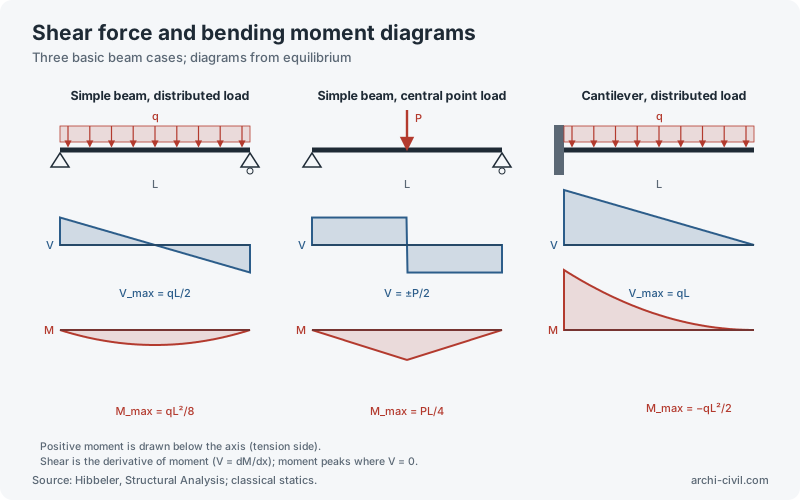
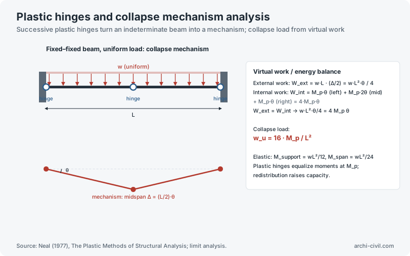
Figure 4.Euler buckling: support conditions and effective lengthFirst buckling modes drawn from the eigenvalue solutionSource: Timoshenko & Gere (1961). K values are theoretical; use code values in design.Open the related tool →Figure 11.Plane stress: Mohr's circlePrincipal stresses and maximum shear stress computed for an example stress stateSource: Mohr (1882); Beer & Johnston, Mechanics of Materials. τ axis drawn positive downward.Open the related tool →Figure 12.Load transfer from slab to beams45° rule: bisectors from the corners divide the slab into tributary areasSource: classical yield-line approach; used with TS 500 and TS 498. Conceptual drawing.Open the related tool →Figure 28.Shear force and bending moment diagramsThree basic beam cases; diagrams from equilibriumSource: Hibbeler, Structural Analysis; classical statics.Open the related tool →Figure 45.Plastic hinges and collapse mechanism analysisSuccessive plastic hinges turn an indeterminate beam into a mechanism; collapse load from virtual workSource: Neal (1977), The Plastic Methods of Structural Analysis; limit analysis.Open the related tool →
Geotechnics and foundations
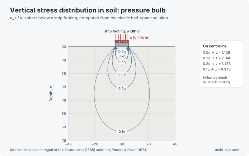
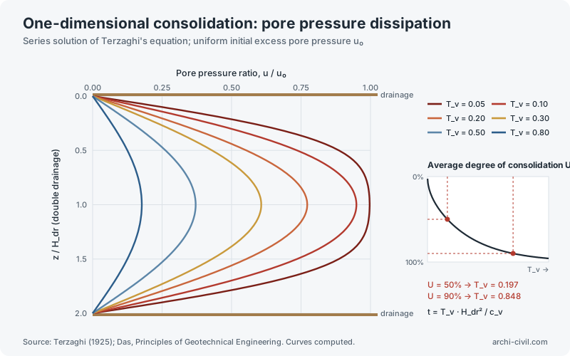
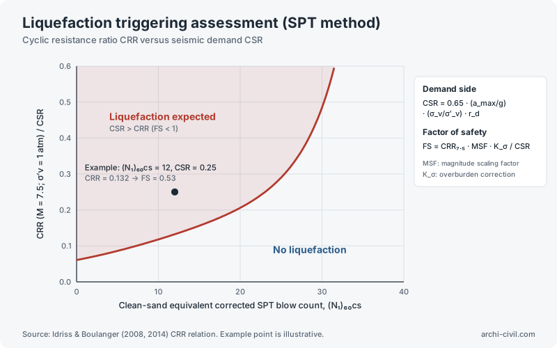
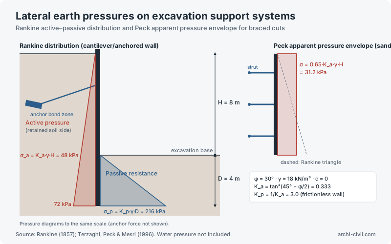
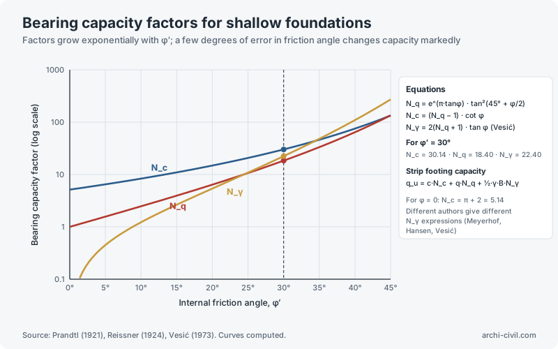
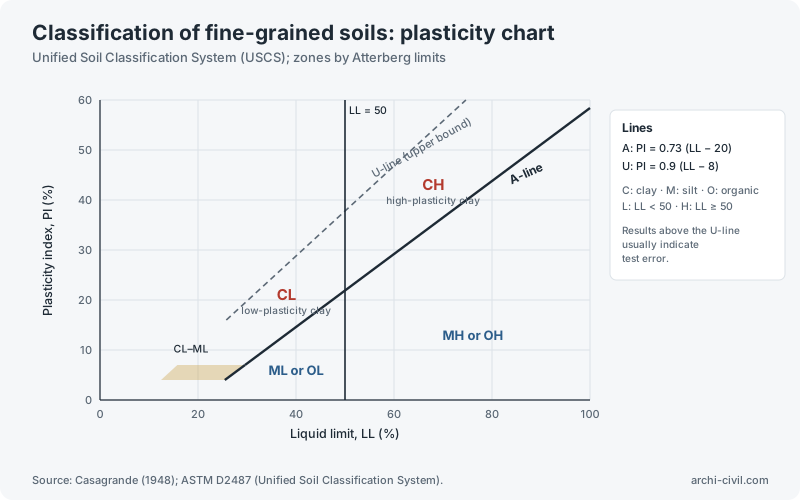
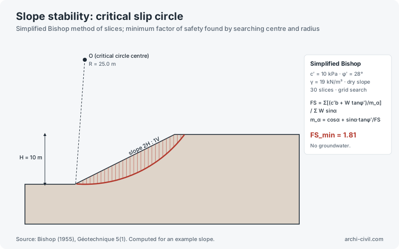
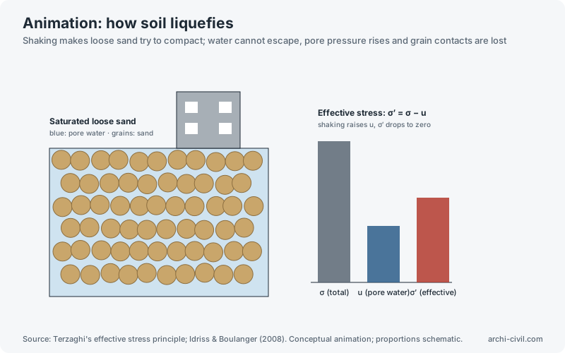
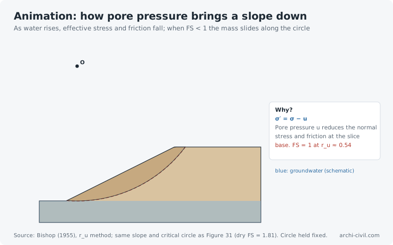
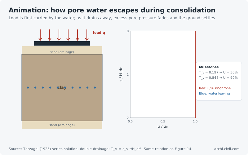
Figure 13.Vertical stress distribution in soil: pressure bulbσ_z / q isobars below a strip footing; computed from the elastic half-space solutionSource: strip-load integral of the Boussinesq (1885) solution; Poulos & Davis (1974).Open the related tool →Figure 14.One-dimensional consolidation: pore pressure dissipationSeries solution of Terzaghi's equation; uniform initial excess pore pressure u₀Source: Terzaghi (1925); Das, Principles of Geotechnical Engineering. Curves computed.Open the related tool →Figure 15.Liquefaction triggering assessment (SPT method)Cyclic resistance ratio CRR versus seismic demand CSRSource: Idriss & Boulanger (2008, 2014) CRR relation. Example point is illustrative.Open the related tool →Figure 22.Lateral earth pressures on excavation support systemsRankine active–passive distribution and Peck apparent pressure envelope for braced cutsSource: Rankine (1857); Terzaghi, Peck & Mesri (1996). Water pressure not included.Open the related tool →Figure 26.Bearing capacity factors for shallow foundationsFactors grow exponentially with φ′; a few degrees of error in friction angle changes capacity markedlySource: Prandtl (1921), Reissner (1924), Vesić (1973). Curves computed.Open the related tool →Figure 30.Classification of fine-grained soils: plasticity chartUnified Soil Classification System (USCS); zones by Atterberg limitsSource: Casagrande (1948); ASTM D2487 (Unified Soil Classification System).Open the related tool →Figure 31.Slope stability: critical slip circleSimplified Bishop method of slices; minimum factor of safety found by searching centre and radiusSource: Bishop (1955), Géotechnique 5(1). Computed for an example slope.Open the related tool →AnimationAnimation A4.How soil liquefiesShaking makes loose sand try to compact; water cannot escape, pore pressure rises and grain contacts are lostSource: Terzaghi's effective stress principle; Idriss & Boulanger (2008). Conceptual animation; proportions schematic.Open the related tool →AnimationAnimation A7.How pore pressure brings a slope downAs water rises, effective stress and friction fall; when FS < 1 the mass slides along the circleSource: Bishop (1955), r_u method; same slope and critical circle as Figure 31 (dry FS = 1.81). Circle held fixed.Open the related tool →AnimationAnimation A8.How pore water escapes during consolidationLoad is first carried by the water; as it drains away, excess pore pressure fades and the ground settlesSource: Terzaghi (1925) series solution, double drainage; T_v = c_v·t/H_dr². Same relation as Figure 14.Open the related tool →
Protective structures
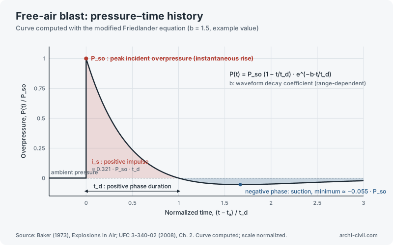
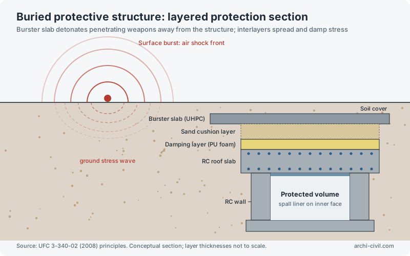
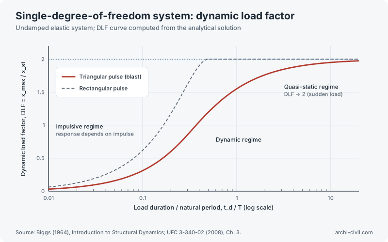
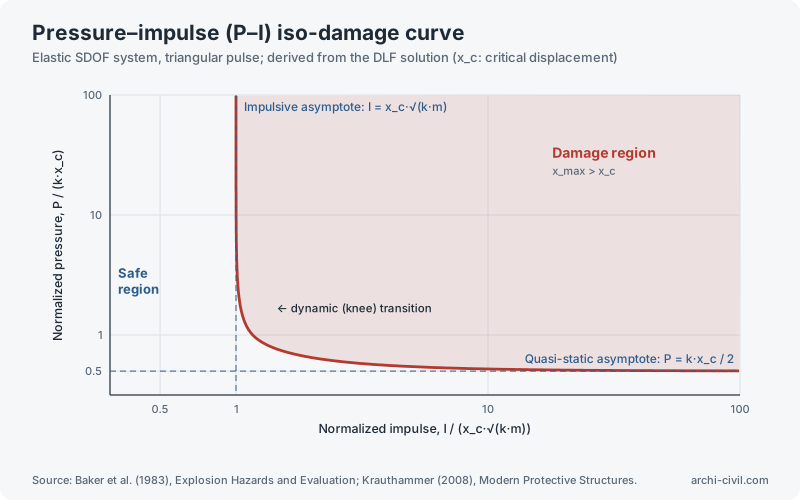
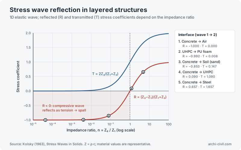
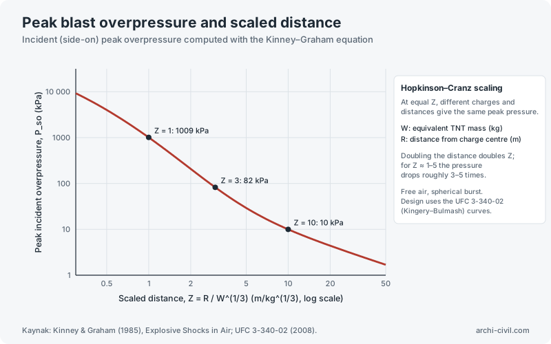
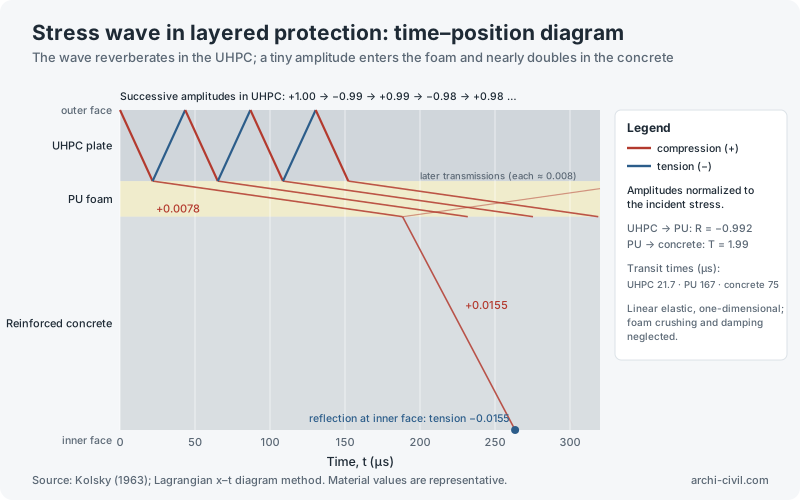
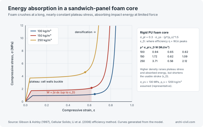
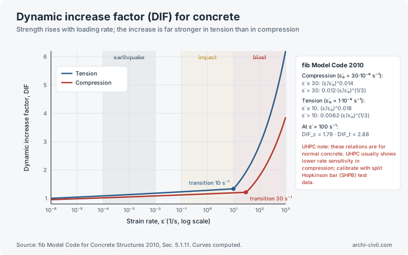
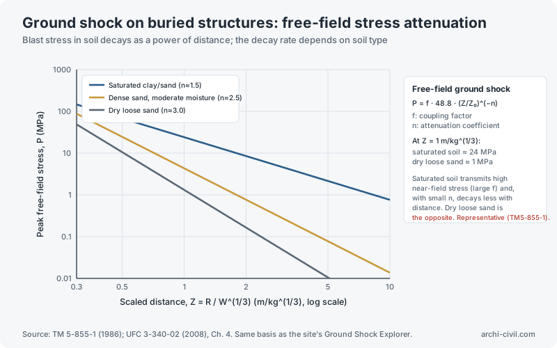
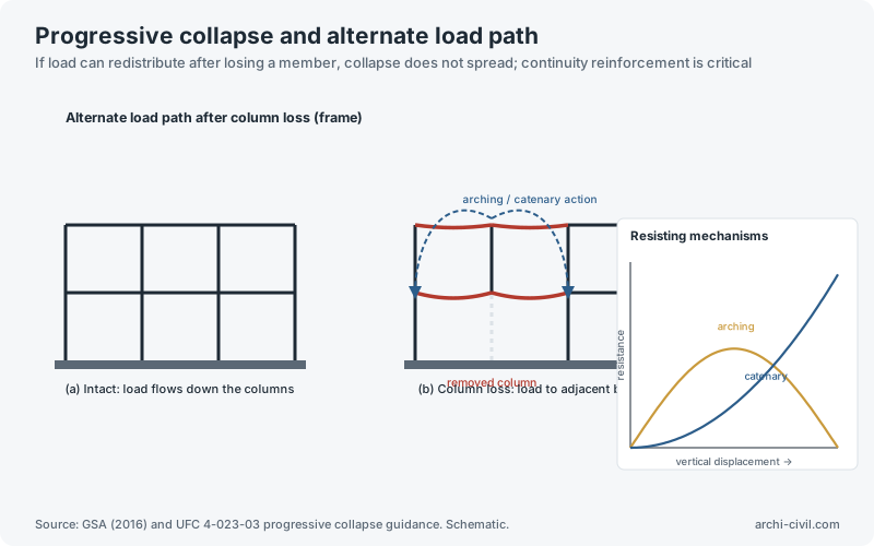
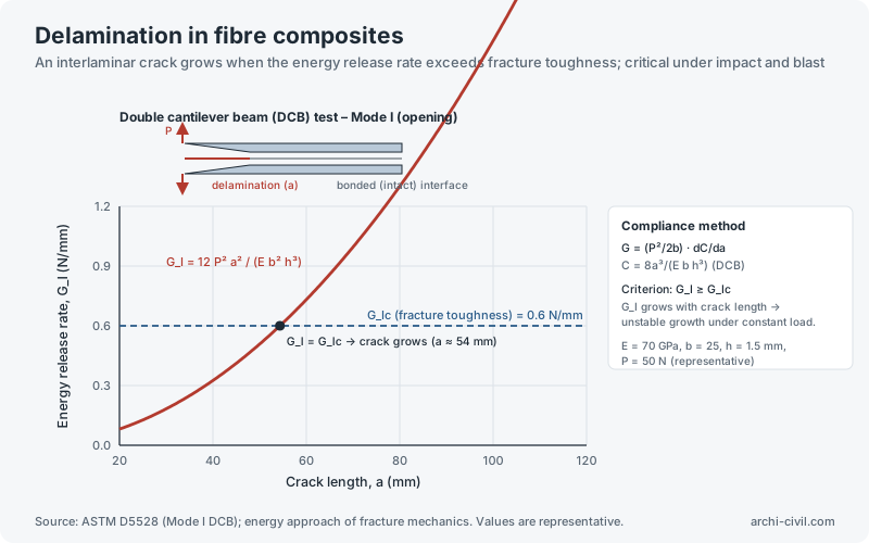
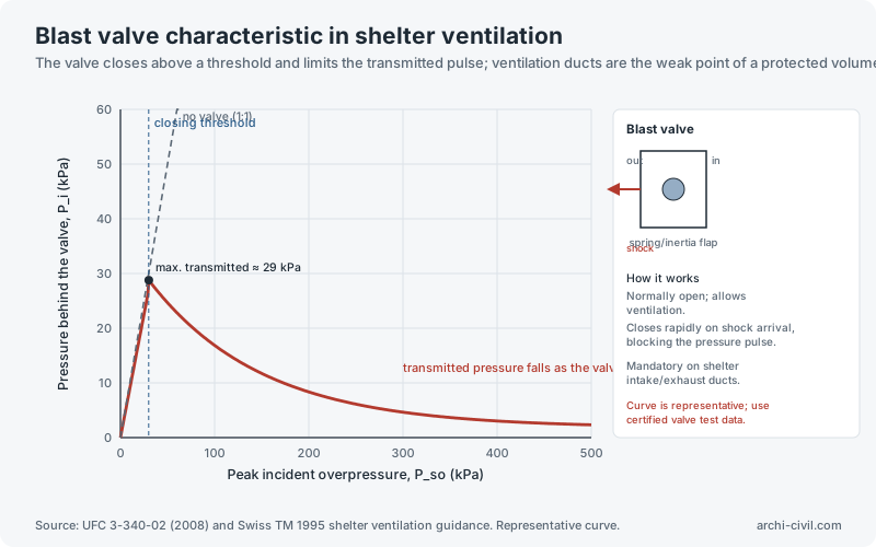
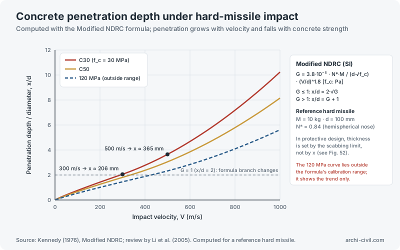
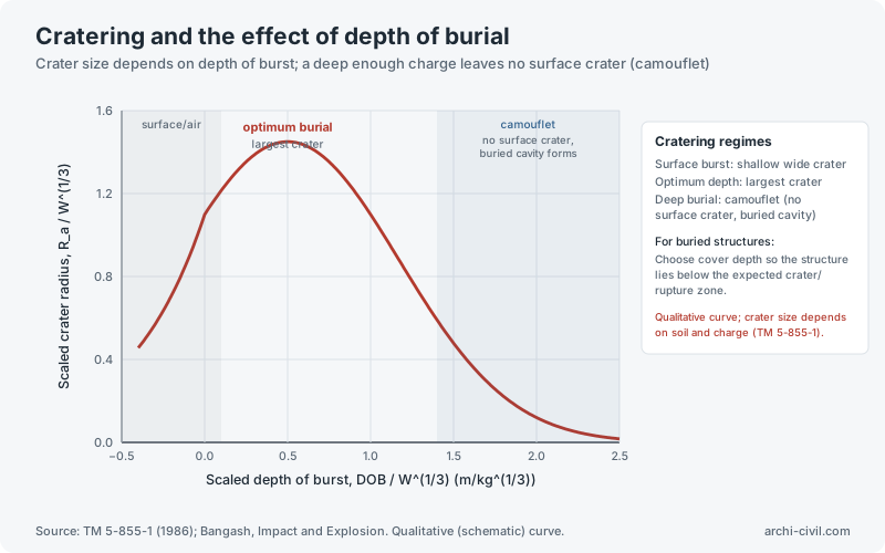
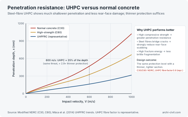
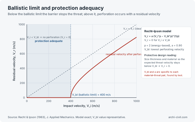
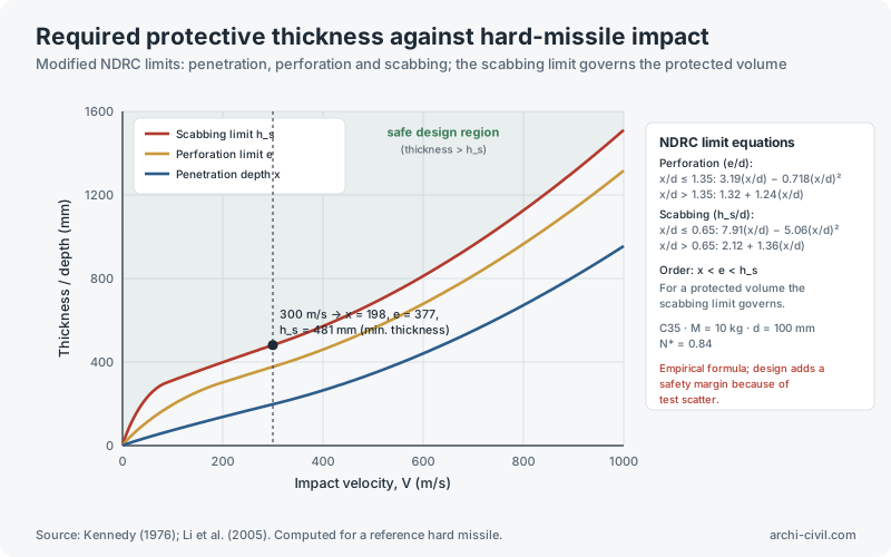
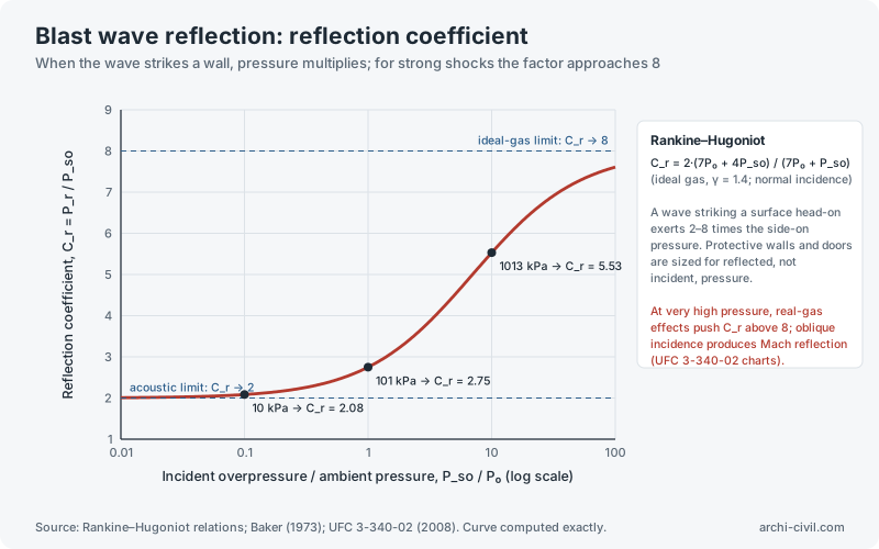
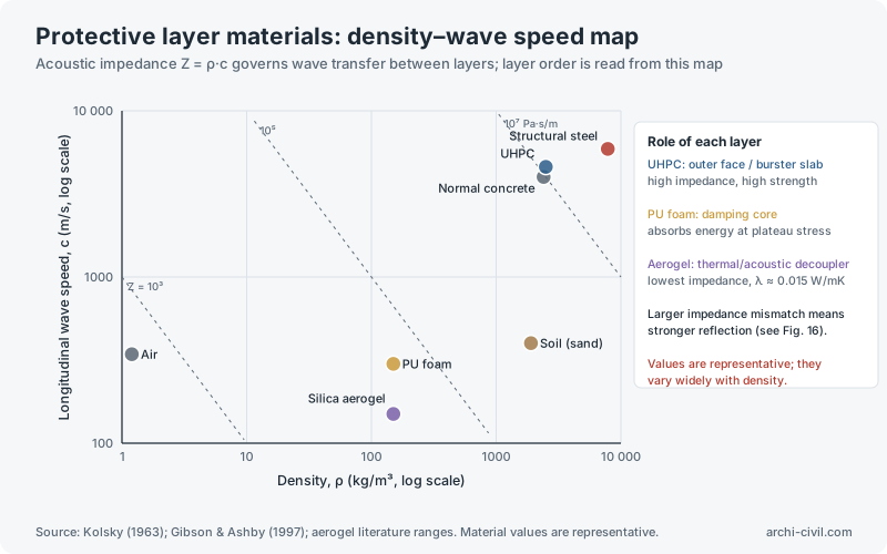
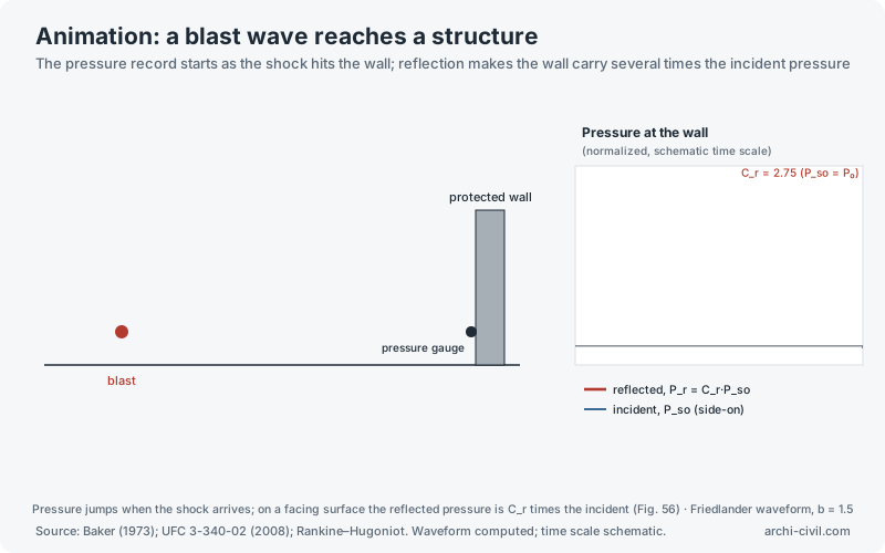
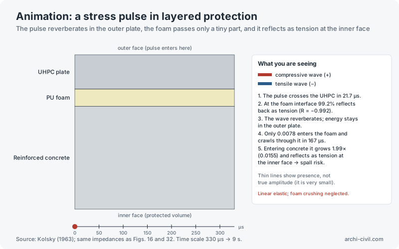
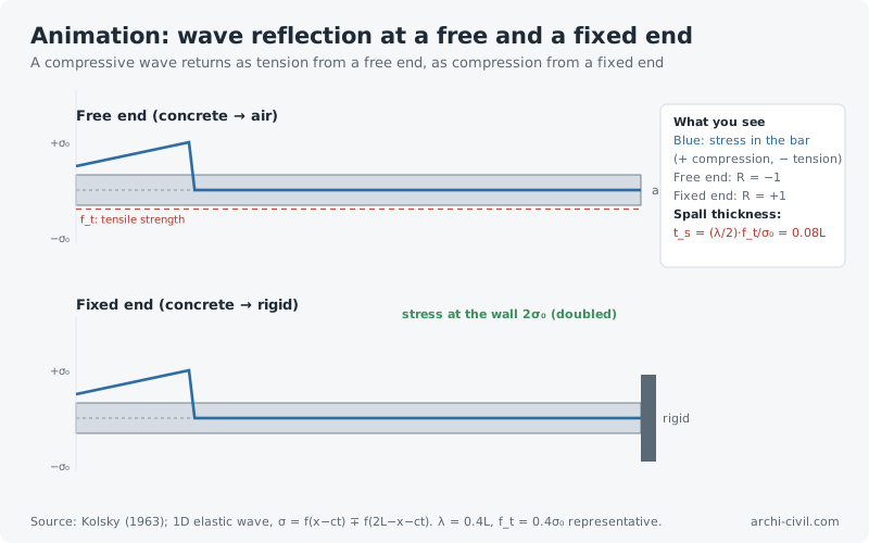
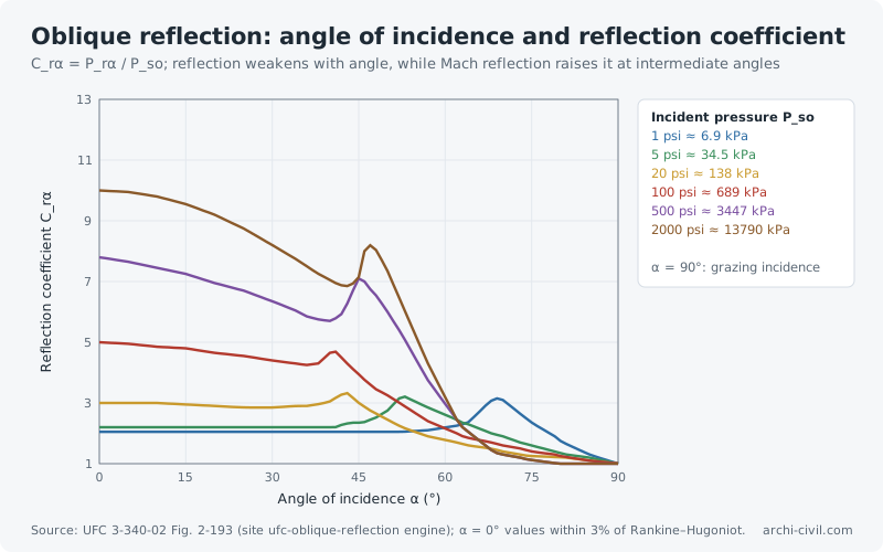
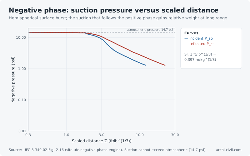
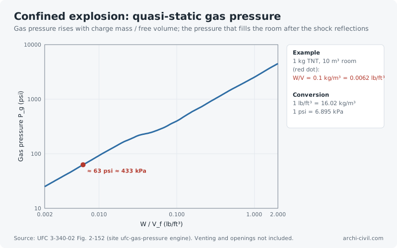
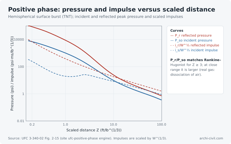
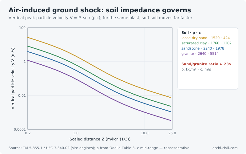
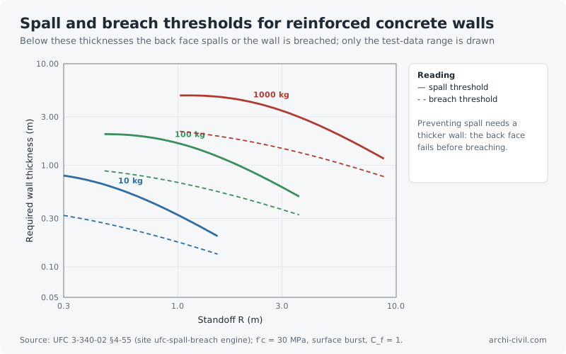
Figure 1.Free-air blast: pressure–time historyCurve computed with the modified Friedlander equation (b = 1.5, example value)Source: Baker (1973), Explosions in Air; UFC 3-340-02 (2008), Ch. 2. Curve computed; scale normalized.Open the related tool →Figure 6.Buried protective structure: layered protection sectionBurster slab detonates penetrating weapons away from the structure; interlayers spread and damp stressSource: UFC 3-340-02 (2008) principles. Conceptual section; layer thicknesses not to scale.Open the related tool →Figure 7.Single-degree-of-freedom system: dynamic load factorUndamped elastic system; DLF curve computed from the analytical solutionSource: Biggs (1964), Introduction to Structural Dynamics; UFC 3-340-02 (2008), Ch. 3.Open the related tool →Figure 8.Pressure–impulse (P–I) iso-damage curveElastic SDOF system, triangular pulse; derived from the DLF solution (x_c: critical displacement)Source: Baker et al. (1983), Explosion Hazards and Evaluation; Krauthammer (2008), Modern Protective Structures.Open the related tool →Figure 16.Stress wave reflection in layered structures1D elastic wave; reflected (R) and transmitted (T) stress coefficients depend on the impedance ratioSource: Kolsky (1963), Stress Waves in Solids. Z = ρ·c; material values are representative.Open the related tool →Figure 27.Peak blast overpressure and scaled distanceIncident (side-on) peak overpressure computed with the Kinney–Graham equationSource: Kinney & Graham (1985), Explosive Shocks in Air; UFC 3-340-02 (2008).Open the related tool →Figure 32.Stress wave in layered protection: time–position diagramThe wave reverberates in the UHPC; a tiny amplitude enters the foam and nearly doubles in the concreteSource: Kolsky (1963); Lagrangian x–t diagram method. Material values are representative.Open the related tool →Figure 36.Energy absorption in a sandwich-panel foam coreFoam crushes at a long, nearly constant plateau stress, absorbing impact energy at limited forceSource: Gibson & Ashby (1997), Cellular Solids; Li et al. (2006) efficiency method. Curves generated from the model.Open the related tool →Figure 37.Dynamic increase factor (DIF) for concreteStrength rises with loading rate; the increase is far stronger in tension than in compressionSource: fib Model Code for Concrete Structures 2010, Sec. 5.1.11. Curves computed.Open the related tool →Figure 40.Ground shock on buried structures: free-field stress attenuationBlast stress in soil decays as a power of distance; the decay rate depends on soil typeSource: TM 5-855-1 (1986); UFC 3-340-02 (2008), Ch. 4. Same basis as the site's Ground Shock Explorer.Open the related tool →Figure 44.Progressive collapse and alternate load pathIf load can redistribute after losing a member, collapse does not spread; continuity reinforcement is criticalSource: GSA (2016) and UFC 4-023-03 progressive collapse guidance. Schematic.Open the related tool →Figure 46.Delamination in fibre compositesAn interlaminar crack grows when the energy release rate exceeds fracture toughness; critical under impact and blastSource: ASTM D5528 (Mode I DCB); energy approach of fracture mechanics. Values are representative.Open the related tool →Figure 47.Blast valve characteristic in shelter ventilationThe valve closes above a threshold and limits the transmitted pulse; ventilation ducts are the weak point of a protected volumeSource: UFC 3-340-02 (2008) and Swiss TM 1995 shelter ventilation guidance. Representative curve.Open the related tool →Figure 48.Concrete penetration depth under hard-missile impactComputed with the Modified NDRC formula; penetration grows with velocity and falls with concrete strengthSource: Kennedy (1976), Modified NDRC; review by Li et al. (2005). Computed for a reference hard missile.Open the related tool →Figure 49.Cratering and the effect of depth of burialCrater size depends on depth of burst; a deep enough charge leaves no surface crater (camouflet)Source: TM 5-855-1 (1986); Bangash, Impact and Explosion. Qualitative (schematic) curve.Open the related tool →Figure 50.Penetration resistance: UHPC versus normal concreteSteel-fibre UHPC shows much shallower penetration and less rear-face damage; thinner protection sufficesSource: Modified NDRC (C30, C80); Máca et al. (2014) UHPFRC trends. UHPC fibre factor is representative.Open the related tool →Figure 51.Ballistic limit and protection adequacyBelow the ballistic limit the barrier stops the threat; above it, perforation occurs with a residual velocitySource: Recht & Ipson (1963), J. Applied Mechanics. Model exact; V_bl value representative.Open the related tool →Figure 52.Required protective thickness against hard-missile impactModified NDRC limits: penetration, perforation and scabbing; the scabbing limit governs the protected volumeSource: Kennedy (1976); Li et al. (2005). Computed for a reference hard missile.Open the related tool →Figure 56.Blast wave reflection: reflection coefficientWhen the wave strikes a wall, pressure multiplies; for strong shocks the factor approaches 8Source: Rankine–Hugoniot relations; Baker (1973); UFC 3-340-02 (2008). Curve computed exactly.Open the related tool →Figure 57.Protective layer materials: density–wave speed mapAcoustic impedance Z = ρ·c governs wave transfer between layers; layer order is read from this mapSource: Kolsky (1963); Gibson & Ashby (1997); aerogel literature ranges. Material values are representative.Open the related tool →AnimationAnimation A2.A blast wave reaches a structureThe pressure record starts as the shock hits the wall; reflection makes the wall carry several times the incident pressureSource: Baker (1973); UFC 3-340-02 (2008); Rankine–Hugoniot. Waveform computed; time scale schematic.Open the related tool →AnimationAnimation A3.A stress pulse in layered protectionThe pulse reverberates in the outer plate, the foam passes only a tiny part, and it reflects as tension at the inner faceSource: Kolsky (1963); same impedances as Figs. 16 and 32. Time scale 330 µs → 9 s.Open the related tool →AnimationAnimation A6.Wave reflection at a free and a fixed endA compressive wave returns as tension from a free end, as compression from a fixed endSource: Kolsky (1963); 1D elastic wave, σ = f(x−ct) ∓ f(2L−x−ct). λ = 0.4L, f_t = 0.4σ₀ representative.Open the related tool →Figure 70.Oblique reflection: angle of incidence and reflection coefficientC_rα = P_rα / P_so; reflection weakens with angle, while Mach reflection raises it at intermediate anglesSource: UFC 3-340-02 Fig. 2-193 (site ufc-oblique-reflection engine); α = 0° values within 3% of Rankine–Hugoniot.Open the related tool →Figure 71.Negative phase: suction pressure versus scaled distanceHemispherical surface burst; the suction that follows the positive phase gains relative weight at long rangeSource: UFC 3-340-02 Fig. 2-16 (site ufc-negative-phase engine). Suction cannot exceed atmospheric (14.7 psi).Open the related tool →Figure 72.Confined explosion: quasi-static gas pressureGas pressure rises with charge mass / free volume; the pressure that fills the room after the shock reflectionsSource: UFC 3-340-02 Fig. 2-152 (site ufc-gas-pressure engine). Venting and openings not included.Open the related tool →Figure 73.Positive phase: pressure and impulse versus scaled distanceHemispherical surface burst (TNT); incident and reflected peak pressure and scaled impulsesSource: UFC 3-340-02 Fig. 2-15 (site ufc-positive-phase engine). Impulses are scaled by W^(1/3).Open the related tool →Figure 74.Air-induced ground shock: soil impedance governsVertical peak particle velocity V = P_so / (ρ·c); for the same blast, soft soil moves far fasterSource: TM 5-855-1 / UFC 3-340-02 (site engines); ρ from Odello Table 3, c mid-range — representative.Open the related tool →Figure 75.Spall and breach thresholds for reinforced concrete wallsBelow these thicknesses the back face spalls or the wall is breached; only the test-data range is drawnSource: UFC 3-340-02 §4-55 (site ufc-spall-breach engine); f′c = 30 MPa, surface burst, C_f = 1.Open the related tool →
Building physics
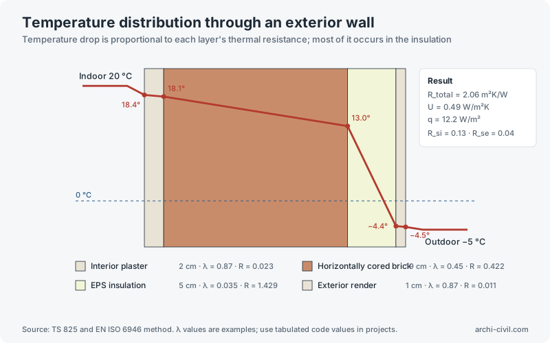
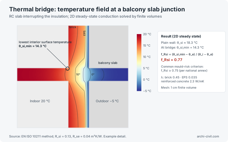
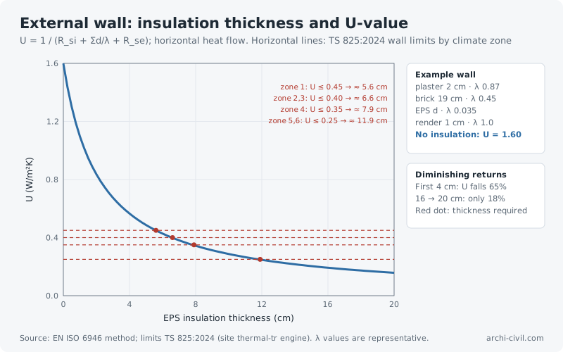
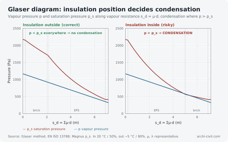
Figure 5.Temperature distribution through an exterior wallTemperature drop is proportional to each layer's thermal resistance; most of it occurs in the insulationSource: TS 825 and EN ISO 6946 method. λ values are examples; use tabulated code values in projects.Open the related tool →Figure 21.Thermal bridge: temperature field at a balcony slab junctionRC slab interrupting the insulation; 2D steady-state conduction solved by finite volumesSource: EN ISO 10211 method; R_si = 0.13, R_se = 0.04 m²K/W. Example detail.Open the related tool →Figure 58.External wall: insulation thickness and U-valueU = 1 / (R_si + Σd/λ + R_se); horizontal heat flow. Horizontal lines: TS 825:2024 wall limits by climate zoneSource: EN ISO 6946 method; limits TS 825:2024 (site thermal-tr engine). λ values are representative.Open the related tool →Figure 59.Glaser diagram: insulation position decides condensationVapour pressure p and saturation pressure p_s along vapour resistance s_d = μ·d; condensation where p > p_sSource: Glaser method, EN ISO 13788; Magnus p_s. In 20 °C / 50%, out −5 °C / 80%. μ, λ representative.Open the related tool →
Site engineering and loads
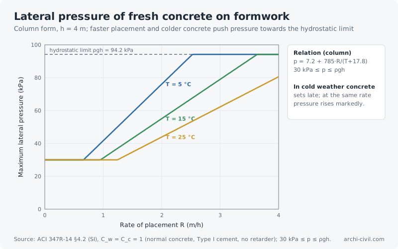
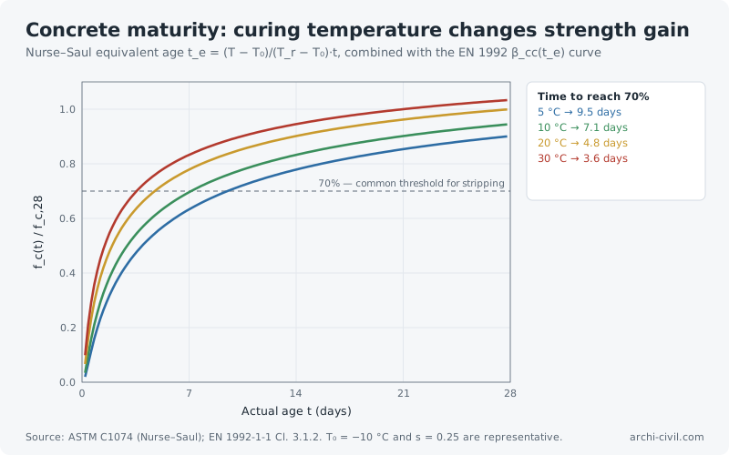
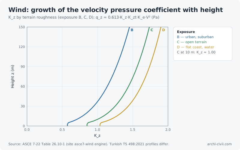
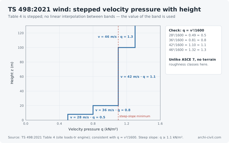
Figure 60.Lateral pressure of fresh concrete on formworkColumn form, h = 4 m; faster placement and colder concrete push pressure towards the hydrostatic limitSource: ACI 347R-14 §4.2 (SI), C_w = C_c = 1 (normal concrete, Type I cement, no retarder); 30 kPa ≤ p ≤ ρgh.Open the related tool →Figure 61.Concrete maturity: curing temperature changes strength gainNurse–Saul equivalent age t_e = (T − T₀)/(T_r − T₀)·t, combined with the EN 1992 β_cc(t_e) curveSource: ASTM C1074 (Nurse–Saul); EN 1992-1-1 Cl. 3.1.2. T₀ = −10 °C and s = 0.25 are representative.Open the related tool →Figure 62.Wind: growth of the velocity pressure coefficient with heightK_z by terrain roughness (exposure B, C, D); q_z = 0.613·K_z·K_zt·K_e·V² (Pa)Source: ASCE 7-22 Table 26.10-1 (site asce7-wind engine). Turkish TS 498:2021 profiles differ.Open the related tool →Figure 69.TS 498:2021 wind: stepped velocity pressure with heightTable 4 is stepped; no linear interpolation between bands — the value of the band is usedSource: TS 498:2021 Table 4 (site loads-tr engine); consistent with q = v²/1600. Steep slope: q ≥ 1.1 kN/m².Open the related tool →
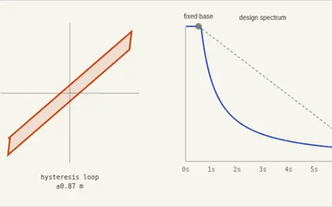 Base Isolation ExplorerInstead of making a building strong enough to survive the shaking, disconnect it from the ground. Lead-rubber bearings lengthen the period far past…
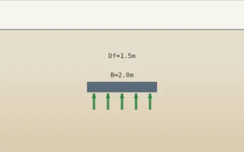 Bearing Capacity ExplorerA shallow foundation, real soil. Change the footing width and embedment depth and watch the allowable bearing pressure respond live — a feel for why…
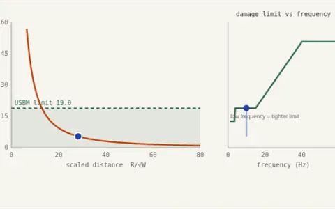 Blast Vibration ControlEvery quarry, tunnel drive and controlled demolition near housing runs into the same limit: not how much rock you can break, but how much the…
 BlastShield Pro 🛡️What happens when a blast wave hits a layered protective wall? You build the layers: ceramic, UHPC, foam, metal… A one-dimensional Lagrangian shock…
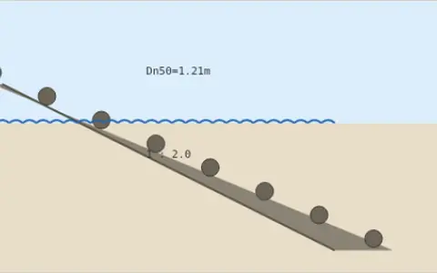 🌊 Breakwater Armor ExplorerA rubble-mound slope, an incoming design wave. Change the wave height and slope and watch the required armor-stone weight respond live — the Hudson…
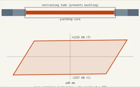 🧱 Buckling-Restrained Brace ExplorerAn ordinary brace buckles in compression, so it is strong one way and weak the other — pinched, lopsided hysteresis. A BRB separates the two jobs: a…
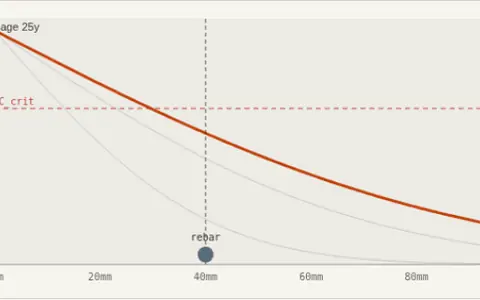 Chloride Service Life ExplorerMost concrete structures don't fail structurally — they corrode out of service decades earlier. Chloride from seawater or de-icing salt diffuses…
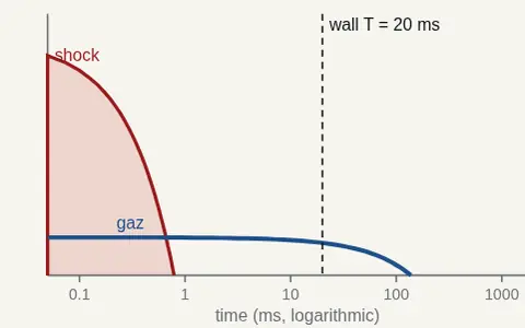 Confined Volume Explorer 🚪🔬Change the charge, the room volume, the opening and the wall freely: watch how shock and gas pressure develop in time and which one loads the wall…
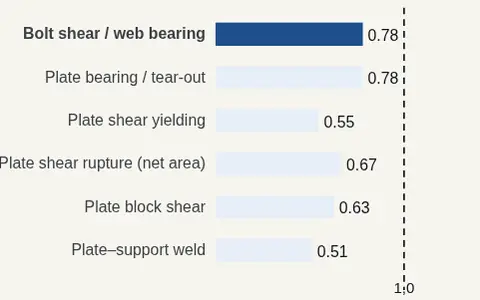 Connection Explorer 🔩🔬Change the number, diameter and grade of the bolts, the plate and the weld freely: watch the ratios of all the connection's limit states and which…
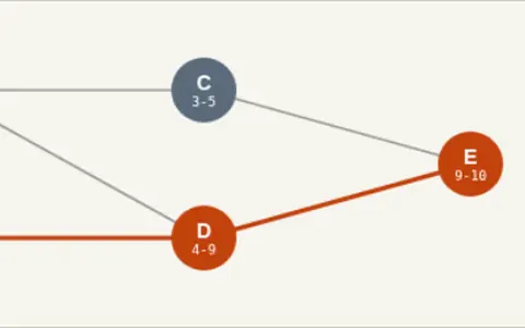 Critical Path ExplorerFive activities, a few dependencies, one project deadline. Change each activity's duration and watch the critical path — the chain of zero-float…
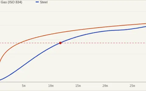 🔥 Fire Resistance ExplorerAn unprotected steel member in a standard fire. Change the section factor (Am/V — how "chunky" the profile is) and the degree of utilisation (how…
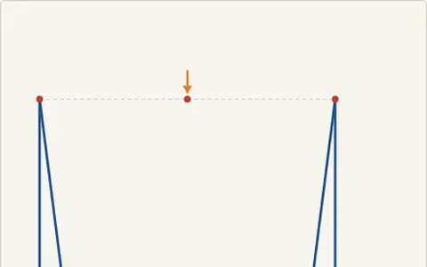 Frame Behavior ExplorerA portal frame — two columns and a beam, both bases fixed. Drag the load's position and change its magnitude and direction, and watch the deflected…
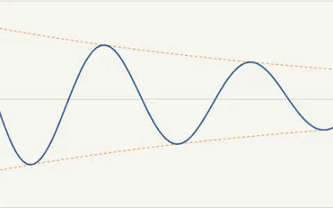 Free Vibration Decay ExplorerPull a structure aside and let it go — no ongoing force, just its own mass, stiffness, and damping deciding what happens next. Change the damping…
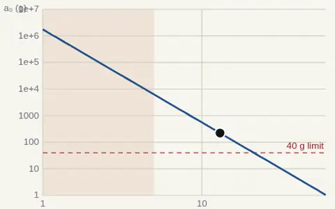 Ground Shock Explorer 🌋A buried or penetrated burst shakes the ground; that shaking reaches the equipment in an underground structure. Change the explosive, the distance…
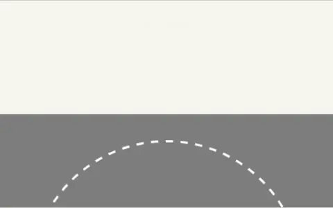 🛣️ Highway Curve ExplorerA car, a banked curve, a speed limit. Change the design speed, superelevation (banking), and side-friction factor and watch the minimum safe curve…
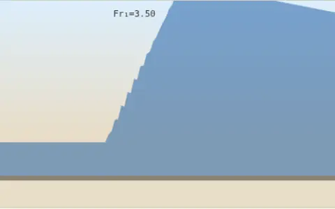 🌀 Hydraulic Jump ExplorerFast, shallow water suddenly slows and piles up. Change the upstream depth and velocity and watch the jump form live — sequent depth, energy…
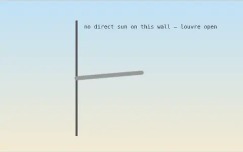 Kinetic Facade ExplorerA motorized horizontal louvre, tracking the sun. Change the date, time, latitude, and the wall's compass orientation, and watch the louvre tilt to…
 Layer Laboratory 🧪🧱Build an envelope of one to three layers freely and press Run: a one-dimensional shock hydrocode computes the stress transmitted to the back face…
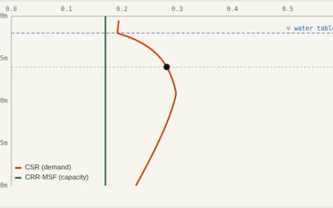 Liquefaction Triggering ExplorerShake loose saturated sand hard enough and pore pressure builds faster than it can drain. Effective stress falls toward zero, and ground that was…
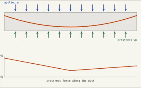 Load Balancing ExplorerT.Y. Lin's insight was to stop thinking about prestress as forces and eccentricities, and start thinking of the curved tendon as a load that pushes…
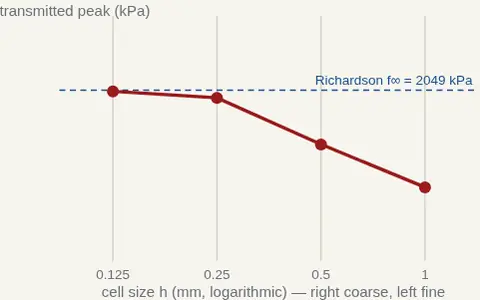 Mesh Convergence 🔬A numerical result is not a result until it stops changing as the mesh is refined. The same layup was solved on successively refined meshes; see the…
 Mode Shape ExplorerA 3-story shear building. Change each story's mass and stiffness and watch the natural frequencies and mode shapes respond instantly. No score, no…
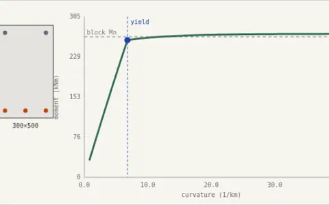 Moment-Curvature ExplorerA rectangular stress block gives you one number: the ultimate moment. A fiber model gives you the whole story — when the steel yields, how far the…
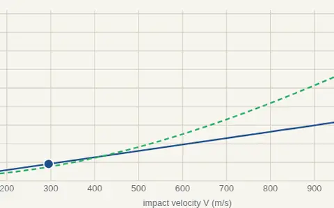 Penetration Explorer 🎯How deep does a projectile penetrate concrete, rock or soil? Where does it stop in a layered protective envelope? Change the projectile, the velocity…
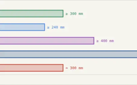 Preliminary Sizing ExplorerOne span, three structural systems. Slide the span and watch how RC beam depth, RC slab thickness, and steel beam depth all scale together in real…
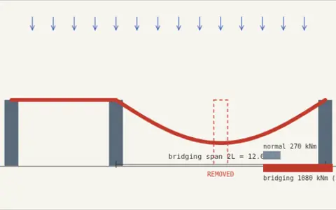 Progressive Collapse ExplorerRemove one column and the beam above it must suddenly span two bays instead of one. Because moment goes with the square of span, the demand jumps by…
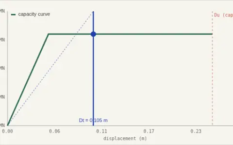 Pushover & Target DisplacementForce-based design asks whether the structure is strong enough. Performance-based design asks a harder question: how far will it actually move, and…
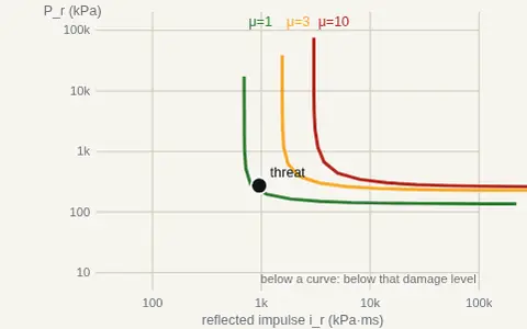 P–I Explorer 🧭Change the wall and the threat freely: the curves of the three damage levels on the pressure–impulse diagram and the position of the threat update…
 Rapid Sizing DrillA random span or story count, one question: what size would you guess? Type your estimate, check it against the standard rule-of-thumb range, then…
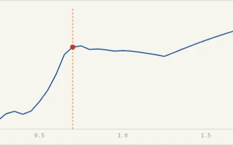 Response Spectrum ExplorerEvery possible structure, one ground motion. Watch a full response spectrum build live as you change damping — the peak response of an SDOF system…
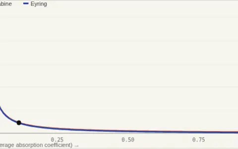 🔊 Reverberation Time ExplorerA room, four surfaces, two competing formulas. Change the finishes (how absorptive floor, ceiling, walls, and windows are) and watch RT60 respond…
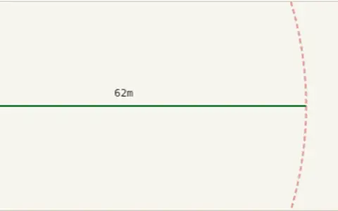 Safe Standoff ExplorerFor accidental-explosion civil protection planning — the kind used around fuel storage, industrial gas facilities, and hazardous material sites.…
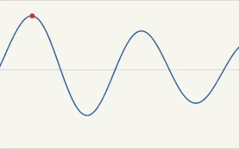 Seismic Response ExplorerA single-degree-of-freedom structure subjected to a ground motion pulse. Change the structure's natural period and damping ratio, and watch how its…
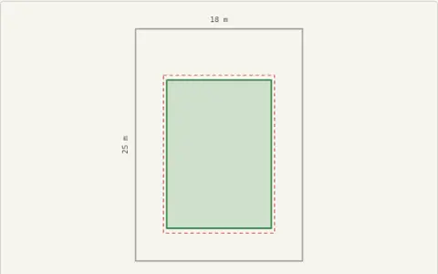 Site Layout ExplorerA rectangular plot, real setback rules, real coverage and floor-area ratios. Change the plot size, setbacks, TAKS (site coverage) and KAKS (floor…
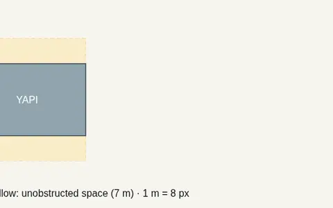 Site Layout Simulation — UFC 4-010-01 Standards 1 and 2Place the installation perimeter, clear zones, building and the objects around it; the standoff (Standard 1) and unobstructed space (Standard 2)…
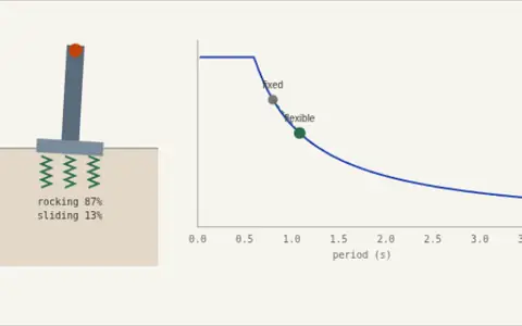 🌍 Soil-Structure Interaction ExplorerA fixed-base model assumes the foundation cannot move. Real soil deforms, adding sliding and rocking springs in series with the structure, and the…
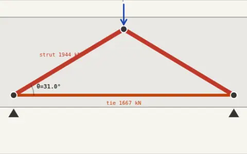 Strut-and-Tie ExplorerNear a support, a deep opening, or a concentrated load, plane sections stop remaining plane and ordinary beam theory quietly stops applying.…
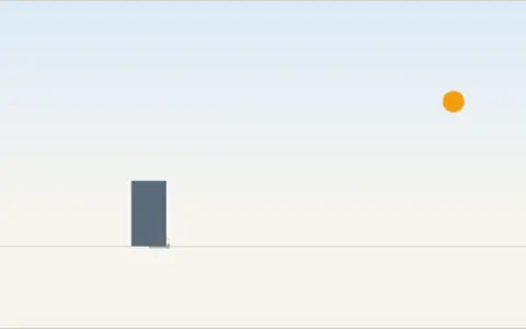 Sun Path & Shadow ExplorerA building, a sun angle, a shadow. Change the date, time of day, and latitude, and watch the shadow stretch, shrink, and swing live — the same real…
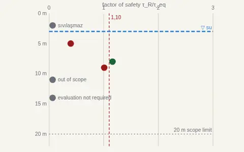 TBDY Liquefaction Profile 🌊🔬Edit the borehole log, add or delete layers, change the earthquake and the groundwater: the TBDY 2018 Annex 16B factor of safety is drawn live along…
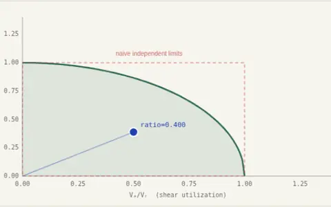 Torsion-Shear InteractionShear and torsion both produce diagonal tension in the web, and on one face they add. A beam comfortably adequate for each action alone can fail…
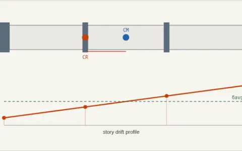 Torsional Irregularity ExplorerPut the stiff core in the middle and the building translates. Push it to one side and the building twists — the far corner takes drift far above the…
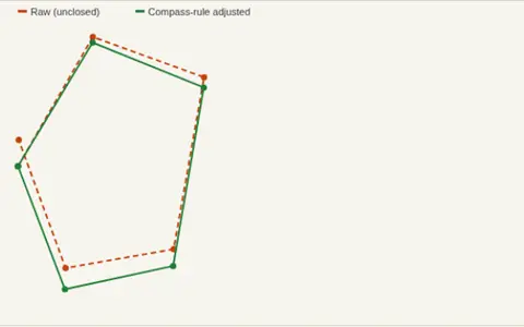 📐 Traverse Closure ExplorerFive legs, a closed loop, a total station. Change each leg's azimuth and distance and watch the polygon fail to close — then watch the compass rule…
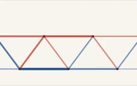 Truss Load Path ExplorerA Warren truss bridge, one moving load. Slide it across the top chord and watch every single member switch between tension (blue) and compression…
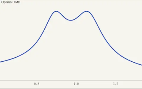 ⚖️ Tuned Mass Damper ExplorerA resonant structure, a small secondary mass on a spring and damper. Change the TMD-to-structure mass ratio and watch Den Hartog's optimal tuning —…
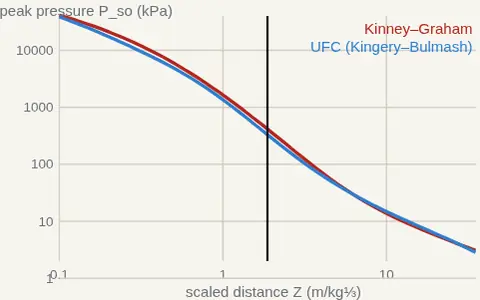 Two Standards ⚖️💥Do two common blast-load models give the same answer to the same question? Change the scaled distance and see where the two models agree and where…
 Wave Journey 🌊💥↓ Visual explanation: 1 figure, 1 animation